Tackling Complex Nonlinear Equations with fzero
The fzero function can handle extremely messy equations — even those mixing exponentials, trigonometric, and logarithmic terms — provided the function is continuous near the root and you give a reasonable starting point or interval.
It’s ideal for cases like:
- Solving energy balance equations
- Finding intersection points of nonlinear models
- Determining parameters from experimental data
Example: Solving for Equilibrium Temperature in a Heat Radiation-Conduction Model
Suppose a spacecraft component exchanges heat via conduction and radiation with its environment. At steady state, the power generated internally equals the heat lost:
Given constants:
 = 25 W
- k = 0.5 W/K
- ϵ = 0.8
- σ = 5.67e−8 W/m²K⁴
- A = 0.1 m²
 = 250 K
Find the steady-state temperature, T.
% Given constants
Qgen = 25;
k = 0.5;
eps = 0.8;
sigma = 5.67e-8;
A = 0.1;
Tinf = 250;
% Define the energy balance equation (set equal to zero)
f = @(T) Qgen - (k*(T - Tinf) + eps*sigma*A*(T.^4 - Tinf^4));
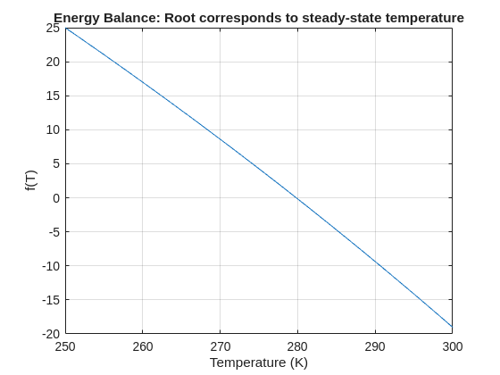
% Plot for a sense of where the root lies before implementing
fplot(f, [250 300]); grid on
xlabel('Temperature (K)'); ylabel('f(T)')
title('Energy Balance: Root corresponds to steady-state temperature')
% Use fzero with an interval that brackets the root
T_eq = fzero(f, [250 300]);
fprintf('Steady-state temperature: %.2f K\n', T_eq);