Dynamic Data Visualization in MATLAB
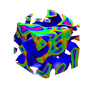
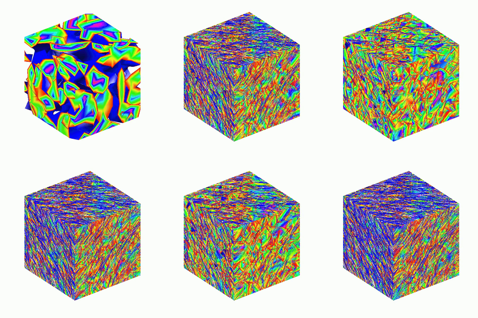
Here presented MATLAB code is designed to create a seamless loop animation that visualizes an isosurface derived from random data.
This entry, titled "The Scrambled Predator's Cube", builds upon my previous work and has been adapted to include dynamic elements.

In this explanation, I will break down the relatively short code, making it accessible whether you are a beginner in MATLAB or an experienced user. Let's go through the MATLAB code step by step to understand each line in detail.
Code Breakdown
d = rand(8,8,8);
Random Data Generation: This line creates a three-dimensional array d with dimensions 8×8×8 filled with random values. The rand function generates values uniformly distributed in the interval (0,1). This array serves as the input data for generating the isosurface.
iv = .5 + (f / 10000);
Isovalue Calculation: Here, the isovalue iv is computed based on the frame number f. The expression f / 10000 causes iv to increase very slowly as f increments. Starting from 0.50, this means that for every increment of f, iv changes slightly (specifically, by 0.0001). This gradual increase creates a smooth transition effect in the isosurface over time, making it look dynamic as the animation progresses.
h = patch(isosurface(d, iv), 'FaceColor', 'blue', 'EdgeColor', 'none');
Isosurface Creation: The isosurface function extracts a 3D surface from the data array d at the specified isovalue iv. The result is a patch object h that represents the isosurface in the 3D plot. The 'FaceColor', 'blue' argument sets the face color of the surface to blue, while 'EdgeColor', 'none' specifies that no edges should be drawn, giving the surface a solid appearance.
isonormals(d, h);
Surface Normals Calculation: This function calculates the normals at each vertex of the isosurface h, based on the data in d. Normals are vectors perpendicular to the surface at each point and are crucial for proper lighting calculations. By using isonormals, the appearance of depth and texture is enhanced, allowing the lighting to interact more realistically with the surface.
patch(isocaps(d, iv), 'FaceColor', 'interp', 'EdgeColor', 'none');
Isocaps Visualization: The isocaps function creates flat surfaces (caps) at the boundaries of the isosurface where the data values meet the isovalue iv. The resulting caps are then rendered as patches with 'FaceColor', 'interp', meaning the colors of the caps are interpolated based on the data values. The caps provide a more complete visual representation of the isosurface, improving its overall appearance.
colormap hsv;
Color Map Setup: This line sets the colormap of the current figure to HSV (Hue, Saturation, Value). The HSV colormap allows for a wide range of colors, which can enhance the visual appeal of the rendering by mapping different values in the data to different colors.
daspect([1, 1, 1]);
Aspect Ratio Setting: The daspect function sets the data aspect ratio of the plot to be equal in all three dimensions. This means that one unit in the x-direction is the same length as one unit in the y-direction and z-direction, ensuring that the visual representation of the 3D data is not distorted.
axis tight;
Tight Axis Setting: This command adjusts the limits of the axes so that they fit tightly around the data, removing any excess white space. It helps to focus the viewer's attention on the isosurface and related visual elements.
view(3);
3D View Configuration: The view(3) command sets the current view to a 3D perspective, allowing the viewer to see the structure of the isosurface from an angle that reveals its three-dimensional nature.
camlight right;
camlight left;
Lighting Effects: These commands add two light sources to the scene, positioned to the right and left of the view. The additional lighting enhances the shading and depth perception of the isosurface, making it appear more three-dimensional and visually appealing.
axis off;
Hide Axes: This command turns off the display of the axes in the plot. Removing the axes provides a cleaner visual representation, allowing the viewer to focus solely on the isosurface and its lighting effects without distraction from the grid lines or axis labels.
lighting phong;
Lighting Model: This line sets the lighting model to Phong. The Phong model is widely used in computer graphics as it provides smooth shading and realistic reflections. It calculates how light interacts with surfaces, enhancing the overall appearance by creating a more natural look.

This code creates a visually dynamic and appealing representation of an isosurface derived from random data. The gradual change in the isovalue allows for smooth transitions, while the combination of lighting, colors, and shading contributes to a rich 3D visualization. Each component plays a vital role in rendering the final output, showcasing advanced techniques in data visualization using MATLAB.
3 Comments
Time DescendingWhat a cool article!!
This is great. Thanks for sharing the tips!
Sign in to participate