Main Content

Results for

Our exportgraphics and copygraphics functions now offer direct and intuitive control over the size, padding, and aspect ratio of your exported figures.
  • Specify Output Size: Use the new Width, Height, and Units name-value pairs
  • Control Padding: Easily adjust the space around your axes using the Padding argument, or set it to to match the onscreen appearance.
  • Preserve Aspect Ratio: Use PreserveAspectRatio='on' to maintain the original plot proportions when specifying a fixed size.
  • SVG Export: The exportgraphics function now supports exporting to the SVG file format.
Check out the full article on the Graphics and App Building blog for examples and details: Advanced Control of Size and Layout of Exported Graphics
Check out how these charts were made with polar axes in the Graphics and App Building blog's latest article "Polar plots with patches and surface".

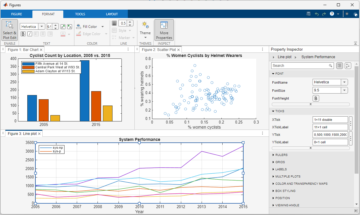
In the latest Graphics and App Building blog article, documentation writer Jasmine Poppick modernized a figure-based bridge analysis app by replacing uicontrol with new UI components and uifigure, resulting in cleaner code, better layouts, and expanded functionality in R2025a.

https://blogs.mathworks.com/graphics-and-apps/2025/08/19/__from-uicontrol-to-ui-components

This article covers the following topics:

Why and when to move from uicontrol and figure to modern UI components and uifigure.

How to replace uicontrol objects with equivalent UI component functions (uicheckbox, uidropdown, uispinner, etc.).

How to update callback code to match new component properties and behaviors.

How to adopt new UI component types (like spinners) to simplify validation and improve usability.

How to configure existing components with modern options (sortable tables, auto-fitting columns, editable data).

How to apply visual styling with uistyle and addStyle to make apps more user-friendly.

How to use uigridlayout to create flexible, adaptive layouts instead of manually managing positions.

The benefits of switching from figure to uifigure for app-building workflows.

A full before-and-after example of modernizing an existing app with incremental, practical updates.

This week's Graphics and App Building blog article guides chart authors and app builders through the process of designing for a specific theme or creating theme-responsive charts and apps.
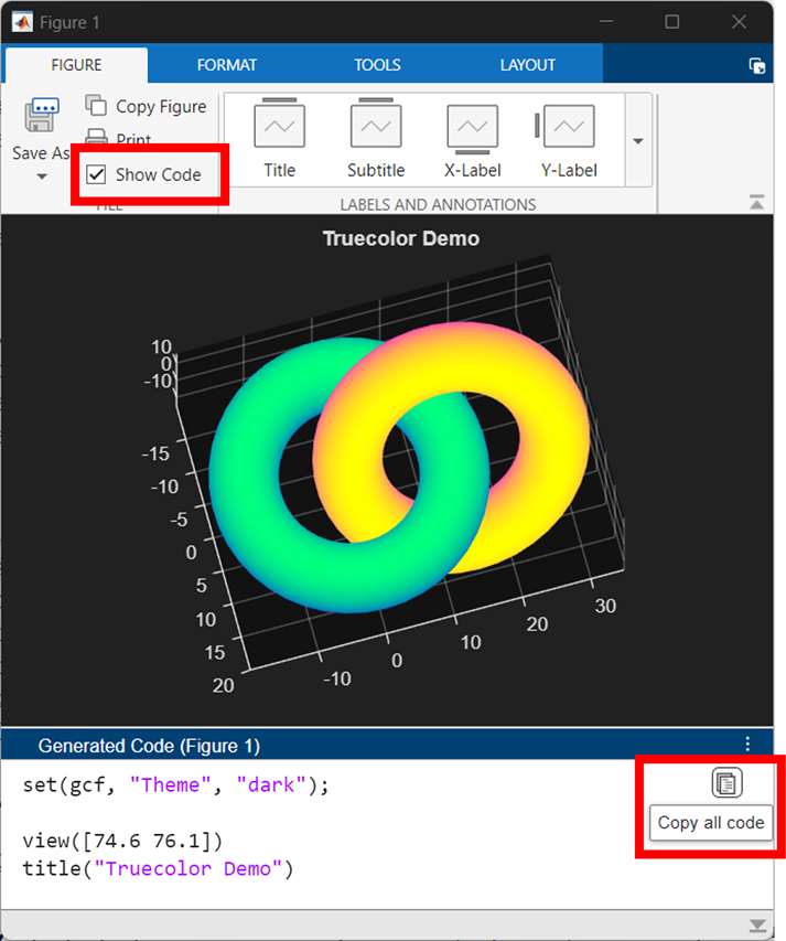
  • Learn how dark theme may impacts charts and apps
  • Discover best practices for theme-adaptive workflows
  • Step-by-step examples for both script-based plots and advanced custom charts and UI components
  • Discover new tools like ThemeChangedFcn, getTheme, and fliplightness
Are you a dark mode enthusiast or are you curious about how it’s shaping MATLAB graphics? Check out the latest article in the MATLAB Graphics and App Building blog.
🔹 User Insights: find out how user surveys influenced the development of graphics themes
🔹 Learn three ways to switch between light and dark themes for figures
🔹 Understand how custom and default colors behave across themes
🔹 Download a handy cheat sheet for working with themes in your graphics and apps.
The new figure toolstrip in R2025a was designed from multiple feedback cycles with MATLAB users. See the latest article in the Graphics and App Building blog to see the evolution of the figure toolbar from 1996-2025, learn how user feedback shaped the new toolstrip, and check out the new code-generation feature that makes interactive data exporation reproducible.
The MATLAB R2025a release gave figures a makeover. @Brian Knolhoff, a developer on the Figure Infrastructure and Services team, reviews the new Figure Container in the Graphics and App Building blog.
Learn the four ways to tile figures, what docking means, and other new features.
The Graphics and App Building Blog just launched its first article on R2025a features, authored by Chris Portal, the director of engineering for the MATLAB graphics and app building teams.
Over the next few months, we'll publish a series of articles that showcase our updated graphics system, introduce new tools and features, and provide valuable references enriched by the perspectives of those involved in their development.
To stay updated, you can subscribe to the blog (look for the option in the upper left corner of the blog page). We also encourage you to join the conversation—your comments and questions under each article help shape the discussion and guide future content.
Do you boast about the energy savings you racking up by using dark mode while stashing your energy bill savings away for an exotic vacation🌴🥥? Well, hold onto your sun hats and flipflops!
A recent study presented at the 1st Internaltional Workshop on Low Carbon Computing suggests that you may be burning more ⚡energy⚡ with your slick dark displays 💻[1].
In a 2x2 factorial design, ten participants viewed a webpage in dark and light modes in both dim and lit settings using an LCD monitor with 16 brightness levels.
  • 80% of participants increased the monitor's brightness in dark mode [2]
  • This occurred in both lit and dim rooms
  • Dark mode did not reduce power draw but increasing monitor brightness did.
The color pixels in an LCD monitor still draw voltage when the screen is black, which is why the monitor looks gray when displaying a pure black background in a dark room. OLED monitors, on the other hand, are capable of turning off pixels that represent pure black and therefore have the potential to save energy with dark mode. A 2021 Purdue study estimates a 3%-9% energy savings with dark mode on OLED monitors using auto-brightness [3]. However, outside of gaming, OLED monitors have a very small market share and still account for less than 25% within the gaming world.
Any MATLAB users out there with OLED monitors? How are you going to spend your mad cash savings when you start using MATLAB's upcoming dark theme?
  1. BBC study: https://www.sicsa.ac.uk/wp-content/uploads/2024/11/LOCO2024_paper_12.pdf
  2. BBC blog article https://www.bbc.co.uk/rd/articles/2025-01-sustainability-web-energy-consumption
  3. 2021 Purdue https://dl.acm.org/doi/abs/10.1145/3458864.3467682
Creating data visualizations
79%
Interpreting data visualizations
21%
28 votes
Three former MathWorks employees, Steve Wilcockson, David Bergstein, and Gareth Thomas, joined the ArrayCast pod cast to discuss their work on array based languages. At the end of the episode, Steve says,
> It's a little known fact about MATLAB. There's this thing, Gareth has talked about the community. One of the things MATLAB did very, very early was built the MATLAB community, the so-called MATLAB File Exchange, which came about in the early 2000s. And it was where people would share code sets, M files, et cetera. This was long before GitHub came around. This was well ahead of its time. And I think there are other places too, where MATLAB has delivered cultural benefits over and above the kind of core programming and mathematical capabilities too. So, you know, MATLAB Central, File Exchange, very much saw the future.
Check out this 3D chart that won Visual Of The Year for 2024 by Visual Capitalist. It's a mashup between a 3D bubblechart and a categorical bar plot yet the only graphical components are the x-axis labels and the legend. Not only does it show relative proportions of material in a laptop but it also shows what the raw material looks like.
I love the idea of analog data visualization. I wonder if any readers have made a analog "chart".
RGB triplet [0,1]
9%
RGB triplet [0,255]
12%
Hexadecimal Color Code
13%
Indexed color
16%
Truecolor array
37%
Equally unfamiliar with all-above
13%
2784 votes
Are you a Simulink user eager to learn how to create apps with App Designer? Or an App Designer enthusiast looking to dive into Simulink?
Don't miss today's article on the Graphics and App Building Blog by @Robert Philbrick! Discover how to build Simulink Apps with App Designer, streamlining control of your simulations!
Welcome to MATLAB Central's first Ask Me Anything (AMA) session! Over the next few weeks, I look forward to addressing any questions or curiosities you might have about MATLAB, the forum, sasquatches, or whatever's on your mind. Having volunteered as a contributor to this community before joining MathWorks, I'm excited to act as a bridge between these two worlds. Let's kick things off by sharing a little-known fact about the forum’s staff contributors!
A couple of years ago, before I joined MathWorks as a developer on the Graphics and Charting team, I often wondered who were the MathWorkers with the [staff] moniker answering questions in the Answers forum. Is their MATLAB Central activity part of their day-to-day job expectations? Do they serve specific roles on some kind of community outreach team? Is their work in the forum voluntary in the same way that non-staff contributors volunteer their time?
Now that I'm on the inside, I'd like to share a secret with my fellow MATLAB users and MATLAB Central enthusiasts: with the exception of the MathWorks Support Team, staff participation in the Answers forum is completely voluntary! The staff contributions you see in the forum arise from pure intrinsic motivation to connect with users, help people out of ruts, and spread the word about our product!
For example, Steven Lord has contributed 20-150 answers per month for 9 years! Steven is a quality engineer for core MATLAB numerical functions. Cris LaPierre develops training material and has been a faithful contributor in the forum for almost 6 years! Kojiro Saito and Akira Agata have been tackling Japanese content for more than 7 years! There are many others who have inspired me as a user, and I am honored to now call colleagues: Peter Perkins, Michio, Joss Knight, Alan Weiss, Jiro Doke, Edric Ellis, and many others who deserve appreciation.
The forum's success hinges on the invaluable contributions from the majority of non-staff volunteers, whose dedication and expertise fuel our community. But I know I wasn't alone in wondering about these staff contributors, so now you're in on the secret!
I'm curious to know what other topics you're interested in learning about. Ask me anything!
I rarely/never save .fig files
47%
Continue working on it later
16%
Archive for future reference
23%
Share within my organization
10%
Share outside my organization
2%
Other (please leave a comment)
2%
2097 votes
Over the weekend I came across a pi approximation using durations of years and weeks (image below, Wolfram, eq. 89), accurate to 6 digits using the average Gregorian year (365.2425 days).
Here it is in MATLAB. I divided by 1 week at the end rather than multiplying by its reciprocal because you can’t divide a numeric by a duration in MATLAB (1/week).
weeks = @(n)n*days(7);
piApprox = ((years(13)-weeks(6))/years(13) + weeks(3)) / weeks(1)
% piApprox = 3.141593493469302
Here’s a breakdown
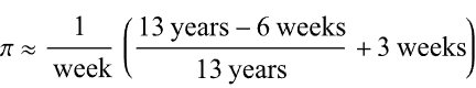
  • The first argument becomes 12.885 yrs / 13 yrs or 0.99115
  • Add three weeks: 0.99115 + 3 weeks = 21.991 days
  • The reduced fraction becomes 21.991 days / 7 days
Now it looks a lot closer to the more familiar approximation for pi 22/7 but with greater precision!
Adam Danz
Adam Danz
Last activity on 6 Mar 2024

I'm curious how the community uses the hold command when creating charts and graphics in MATLAB. In short, hold on sets up the axes to add new objects to the axes while hold off sets up the axes to reset when new objects are added.
When you use hold on do you always follow up with hold off? What's your reasoning on this decision?
Can't wait to discuss this here! I'd love to hear from newbies and experts alike!
figure out what my old code does
18%
write code comments for future me
11%
address a code analyzer warning
3%
reflect on the skills I've gained
8%
get food on my mouse and keyboard
38%
All of the above
22%
16434 votes
New in R2022b: GridSizeChangedFcn
tiledlayout() creates a TiledChartLayout object that defines a gridded layout of axes within a figure. When using the 'flow' option, the grid size becomes dynamic and updates as axes are added or as the figure size changes. These features were introduced in R2019b and if you're still stuck on using subplot, you're missing out on several other great features of tiledlayout.
Starting in MATLAB R2022b you can define a callback function that responds to changes to the grid size in flow arrangements by setting the new gridSizeChangedFcn.
Use case
I often use a global legend to represent data across all axes within a figure. When the figure is tall and narrow, I want the legend to be horizontally oriented at the bottom of the figure but when the figure is short and wide, I prefer a vertically oriented legend on the right of the figure. By using the gridSizeChangedFcn, now I can update the legend location and orientation when the grid size changes.
Demo
gridSizeChangeFcn works like all other graphics callback functions. In this demo, I've named the gridSizeChangedFcn "updateLegendLayout", assigned by an anonymous function. The first input is the TiledChartLayout object and the second input is the event object that indicates the old and new grid sizes. The legend handle is also passed into the function. Since all of the tiles contain the same groups of data, the legend is based on data in the last tile.
As long as the legend is valid, the gridSizeChangedFcn updates the location and orientation of the legend so that when the grid is tall, the legend will be horizontal at the bottom of the figure and when the grid is wide, the legend will be vertical at the right of the figure.
Since the new grid size is available as a property in the TiledChartLayout object, I chose not to use the event argument. This way I can directly call the callback function at the end to update the legend without having to create an event.
Run this example from an m-file. Then change the width or height of the figure to demonstrate the legend adjustments.
% Prepare data
data1 = sort(randn(6))*10;
data2 = sort(randn(6))*10;
labels = ["A","B","C","D","E","F"];
groupLabels = categorical(["Control", "Test"]);
% Generate figure
fig = figure;
tcl = tiledlayout(fig, "flow", TileSpacing="compact", Padding="compact");
nTiles = height(data1);
h = gobjects(1,nTiles);
for i = 1:nTiles
ax = nexttile(tcl);
groupedData = [data1(i,:); data2(i,:)];
h = bar(ax,groupLabels, groupedData, "grouped");
title(ax,"condition " + i)
end
title(tcl,"GridSizeChangedFcn Demo")
ylabel(tcl,"Score")
legh = legend(h, labels);
title(legh,"Factors")
% Define and call the GridSizeChangeFcn
tcl.GridSizeChangedFcn = @(tclObj,event)updateLegendLayout(tclObj,event,legh);
updateLegendLayout(tcl,[],legh);
% Manually resize the vertical and horizontal dimensions of the figure
function updateLegendLayout(tclObj,~,legh)
% Evoked when the TiledChartLayout grid size changes in flow arrangements.
% tclObj - TiledChartLayout object
% event - (unused in this demo) contains old and new grid size
% legh - legend handle
if isgraphics(legh,'legend')
if tclObj.GridSize(1) > tclObj.GridSize(2)
legh.Layout.Tile = "south";
legh.Orientation = "horizontal";
else
legh.Layout.Tile = "east";
legh.Orientation = "vertical";
end
end
end
Give it a shot in MATLAB R2022b
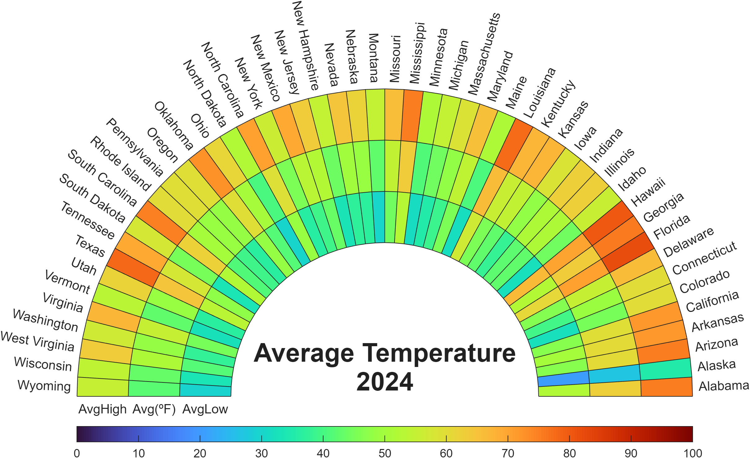
  • Replace the legend with a colorbar to update the location and orientation of the colorbar.
  • Define a GridSizeChangedFcn within the loop so that it is called every time a tile is added.
  • Create a figure with many tiles (~20) and dynamically set a color to each row of axes.
  • Assign xlabels only to the bottom row of tiles and ylabels to only the left column of tiles.
Learn about other new features
This article is attached as a live script.