Walkthrough: making Little Nemo's airship in Matlab
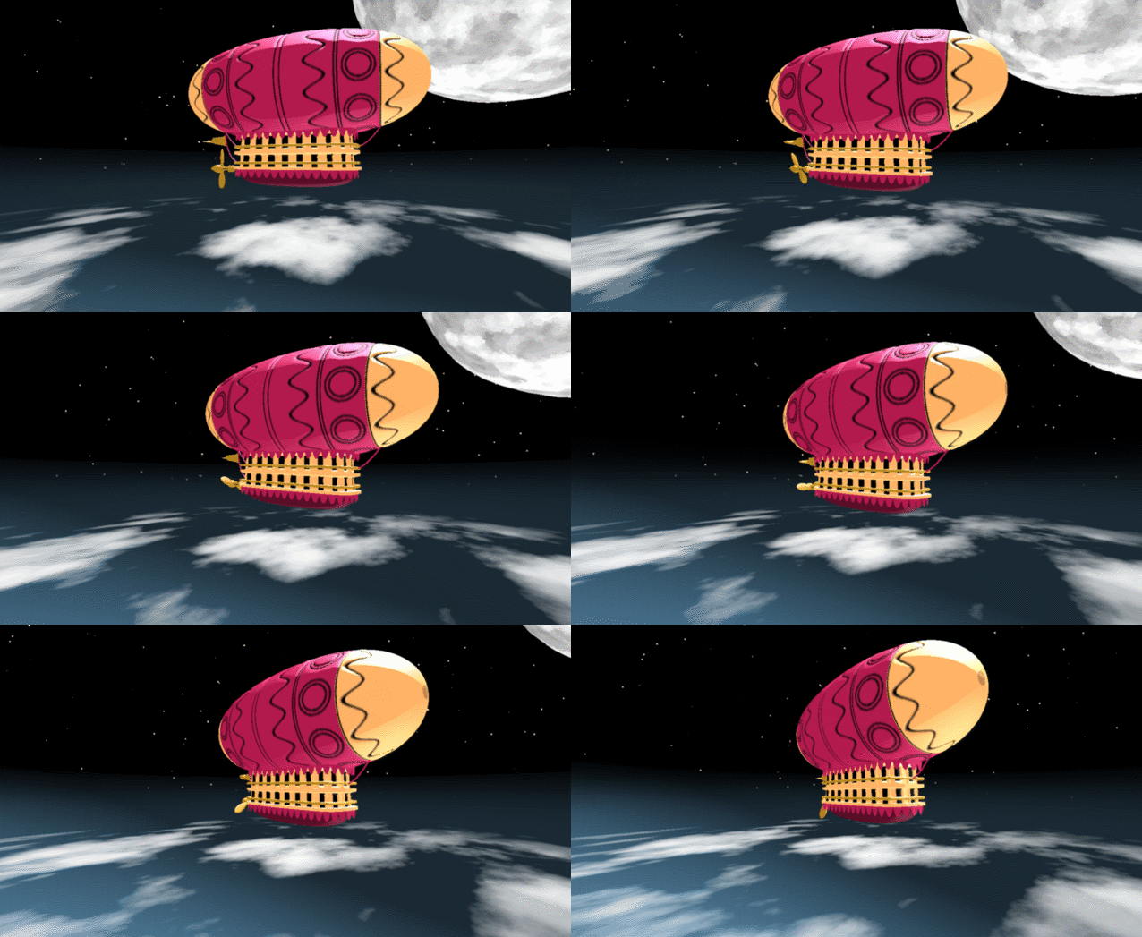
In the spirit of warming up for this year's minihack contest, I'm uploading a walkthrough for how to design an airship using pure Matlab script. This is commented and uncondensed; half of the challenge for the minihacks is how minimize characters. But, maybe it will give people some ideas.
The actual airship design is from one of my favorite original NES games that I played when I was a kid - Little Nemo: The Dream Master. The design comes from the intro of the game when Nemo sees the Slumberland airship leave for Slumberland:
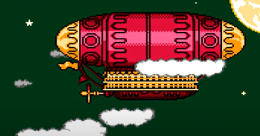
(Snip from a frame of the opening scene in Capcom's game Little Nemo: The Dream Master, showing the Slumberland airship).
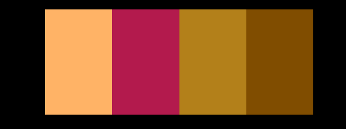
I spent hours playing this game with my two sisters, when we were little. It's fun and tough, but the graphics sparked the imagination. On to the code walkthrough, beginning with the color palette: these four colors are the only colors used for the airship:
c1=cat(3,1,.7,.4); % Cream color
c2=cat(3,.7,.1,.3); % Magenta
c3=cat(3,0.7,.5,.1); % Gold
c4=cat(3,.5,.3,0); % bronze
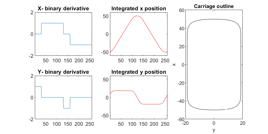
We start with the airship carriage body. We want something rectangular but smoothed on the corners. To do this we are going to start with the separate derivatives of the x and y components, which can be expressed using separate blocks of only three levels: [1, 0, -1]. You could integrate to create a rectangle, but if we smooth the derivatives prior to integrating we will get rounded edges. This is done in the following code:
% Binary components for x & y vectors
z=zeros(1,30);
o=ones(1,100);
% X and y vectors
x=[z,o,z,-o];
y=[1+z,1-o,z-1,1-o];
% Smoother function (fourier / circular)
s=@(x)ifft(fft(x).*conj(fft(hann(45)'/22,260)));
% Integrator function with replication and smoothing to form mesh matrices
u=@(x)repmat(cumsum(s(x)),[30,1]);
% Construct x and y components of carriage with offsets
x3=u(x)-49.35;
y3=u(y)+6.35;
y3 = y3*1.25; % Make it a little fatter
% Add a z-component to make the full set of matrices for creating a 3D
% surface:
z3=linspace(0,1,30)'.*ones(1,260)*30;
z3(14,:)=z3(15,:); % These two lines are for adding platforms
z3(2,:)=z3(3,:); % to the carriage, later.
Plotting x, y, and the top row of the smoothed, integrated, and replicated matrices x3 and y3 gives the following:
We now have the x and y components for a 3D mesh of the carriage, let's make it more interesting by adding a color scheme including doors, and texture for the trim around the doors. Let's also add platforms beneath the doors for passengers to walk on.
Starting with the color values, let's make doors by convolving points in a color-matrix by a door shaped function.
m=0*z3; % Image matrix that will be overlayed on carriage surface
m(7,10:12:end)=1; % Door locations (lower deck)
m(21,10:12:end)=1; % Door locations (upper deck)
drs = ones(9, 5); % Door shape
m=1-conv2(m,ones(9,5),'same'); % Applying
To add the trim, we will convolve matrix "m" (the color matrix) with a square function, and look for values that lie between the extrema. We will use this to create a displacement function that bumps out the -x, and -y values of the carriage surface in intermediary polar coordinate format.
rm=conv2(m,ones(5)/25,'same'); % Smoothing the door function
rm(~m)=0; % Preserving only the region around the doors
rds=0*m; % Radial displacement function
rds(rm<1&rm>0)=1; % Preserving region around doors
rds(m==0)=0;
rds(13:14,:)=6; % Adding walkways
rds(1:2,:)=6;
% Apply radial displacement function
[th,rd]=cart2pol(x3,y3);
[x3T,y3T]=pol2cart(th,(rd+rds)*.89);
If we plot the color function (m) and radial displacement function (rds) we get the following:
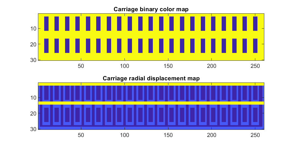
In the upper plot you can see the doors, and in the bottom map you can see the walk way and door trim.
Next, we are going to add some flags draped from the bottom and top of the carriage. We are going to recycle the values in "z3" to do this, by multiplying that matrix with the absolute value of a sine-wave, squished a bit with the soft-clip erf() function.
We add a keel to the airship carriage using a canonical sphere turned on its side, again using the soft-clip erf() function to make it roughly rectangular in x and y, and multiplying with a vector that is half nan's to make the top half transparent.
At this point, since we are beginning the plotting of the ship, we also need to create our hgtransform objects. These allow us to move all of the components of the airship in unison, and also link objects with pivot points to the airship, such as the propeller.
% Now we need some flags extending around the top and bottom of the
% carriage. We can do this my multiplying the height function (z3) with the
% absolute value of a sine-wave, rounded with a compression function
% (erf() in this case);
g=-z3.*erf(abs(sin(linspace(0,40*pi,260))))/4; % Flags
% Also going to add a slight taper to the carriage... gives it a nice look
tp=linspace(1.05,1,30)';
% Finally, plotting. Plot the carriage with the color-map for the doors in
% the cream color, than the flags in magenta. Attach them both to transform
% objects for movement.
% Set up transform objects. 2 moving parts:
% 1) The airship itself and all sub-components
% 2) The propellor, which attaches to the airship and spins on its axis.
hold on;
P=hgtransform('Parent',gca); % Ship
S=hgtransform('Parent',P); % Prop
surf(x3T.*tp,y3T,z3,c1.*m,'Parent',P);
surf(x3,y3,g,c2.*rd./rd, 'Parent', P);
surf(x3,y3,g+31,c2.*rd./rd, 'Parent', P);
axis equal
% Now add the keel of the airship. Will use a canonical sphere and the
% erf() compression function to square off.
[x,y,z]=sphere(99);
mk=round(linspace(-1,1).^2+.3); % This function makes the top half of the sphere nan's for transparency.
surf(50*erf(1.4*z),15*erf(1.4*y),13*x.*mk./mk-1,.5*c2.*z./z, 'Parent', P);
% The carriage is done. Now we can make the blimp above it.
We haven't adjusted the shading of the image yet, but you can see the design features that have been created:
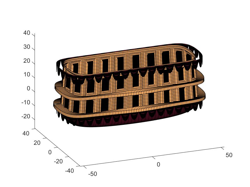
Next, we start working on the blimp. This is going to use a few more vertices & faces. We are going to use a tapered cylinder for this part, and will start by making the overlaid image, which will have 2 colors plus radial rings, circles, and squiggles for ornamentation.
M=525; % Blimp (matrix dimensions)
N=700;
% Assign the blimp the cream and magenta colors
t=122; % Transition point
b=ones(M,N,3); % Blimp color map template
bc=b.*c1; % Blimp color map
bc(:,t+1:end-t,:)=b(:,t+1:end-t,:).*c2;
% Add axial rings around blimp
l=[.17,.3,.31,.49];
l=round([l,1-fliplr(l)]*N); % Mirroring
lnw=ones(1,N); % Mask
lnw(l)=0;
lnw=rescale(conv(lnw,hann(7)','same'));
bc=bc.*lnw;
% Now add squiggles. We're going to do this by making an even function in
% the x-dimension (N, 725) added with a sinusoidal oscillation in the
% y-dimension (M, 500), then thresholding.
r=sin(linspace(0, 2*pi, M)*10)'+(linspace(-1, 1, N).^6-.18)*15;
q=abs(r)>.15;
r=sin(linspace(0, 2*pi, M)*12)'+(abs(linspace(-1, 1, N))-.25)*15;
q=q.*(abs(r)>.15);
% Now add the circles on the blimp. These will be spaced evenly in the
% polar angle dimension around the axis. We will have 9. To make the
% circles, we will create a cone function with a peak at the center of the
% circle, and use thresholding to create a ring of appropriate radius.
hs=[1,.75,.5,.25,0,-.25,-.5,-.75,-1]; % Axial spacing of rings
% Cone generation and ring loop
xy= @(h,s)meshgrid(linspace(-1, 1, N)+s*.53,(linspace(-1, 1, M)+h)*1.15);
w=@(x,y)sqrt(x.^2+y.^2);
for n=1:9
h=hs(n);
[xx,yy]=xy(h,-1);
r1=w(xx,yy);
[xx,yy]=xy(h,1);
r2=w(xx,yy);
b=@(x,y)abs(y-x)>.005;
q=q.*b(.1,r1).*b(.075,r1).*b(.1,r2).*b(.075,r2);
end
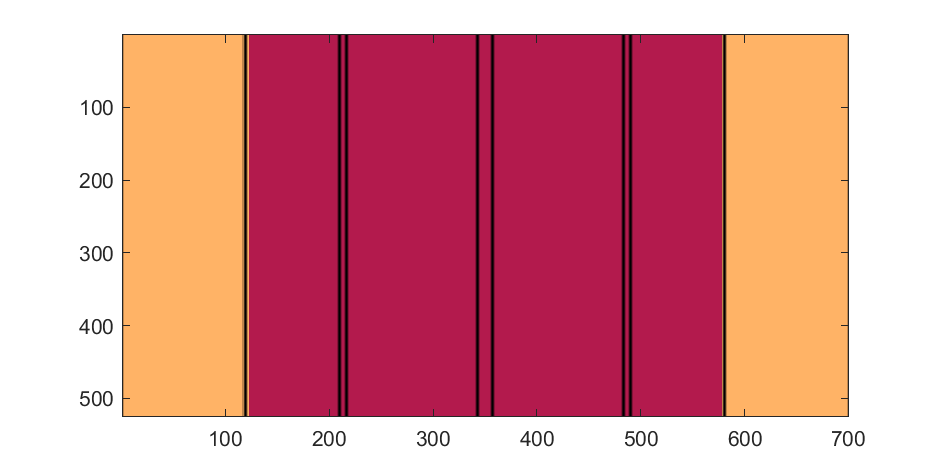
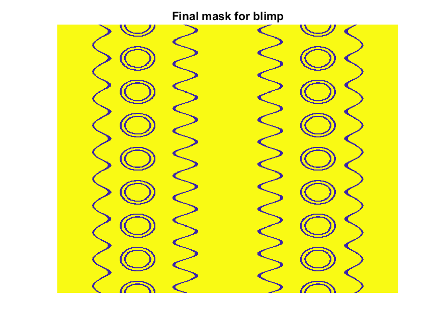
The figures below show the color scheme and mask used to apply the squiggles and circles generated in the code above:
Finally, for the colormap we are going to smooth the binary mask to avoid hard transitions, and use it to to add a "puffy" texture to the blimp shape. This will be done by diffusing the mask iteratively in a loop with a non-linear min() operator.
% 2D convolution function
ff=@(x)circshift(ifft2(fft2(x).*conj(fft2(hann(7)*hann(7)'/9,M,N))),[3,3]);
q=ff(q); % Smooth our mask function
hh=rgb2hsv(q.*bc); % Convert to hsv: we are going to use the value
% component for radial displacement offsets of the
% 3D blimp structure.
rd=hh(:,:,3); % Value component
for n=1:10
rd=min(rd,ff(rd)); % Diffusing the value component for a puffy look
end
rd=(rd+35)/36; % Make displacements effects small
% Now make 3D blimp manifold using "cylinder" canonical shape
[x,y,z]=cylinder(erf(sin(linspace(0,pi,N)).^.5)/4,M-1); % First argument is the blimp taper
[t,r]=cart2pol(x, y);
[x2,y2]=pol2cart(t, r.*rd'); % Applying radial displacment from mask
s=200;
% Plotting the blimp
surf(z'*s-s/2, y2'*s, x2'*s+s/3.9+15, q.*bc,'Parent',P);
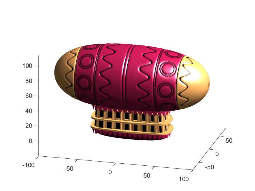
Notice that the parent of the blimp surface plot is the same as the carriage (e.g. hgtransform object "P"). Plotting at this point using flat shading and adding some lighting gives the image below:
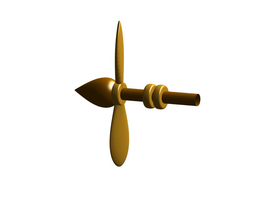
Next, we need to add a propeller so it can move. This will include the creation of a shaft using the cylinder() function. The rest of the pieces (the propeller blades, collars and shaft tip) all use the same canonical sphere with distortions applied using various math functions. Note that when the propeller is made it is linked to hgtransform object "S" rather than "P." This will allow the propeller to rotate, but still be joined to the airship.
% Next, the propeller. First, we start with the shaft. This is a simple
% cylinder. We add an offset variable and a scale variable to move our
% propeller components around, as well.
shx = -70; % This is our x-shifter for components
scl = 3; % Component size scaler
[x,y,z]=cylinder(1, 20); % Canonical cylinder for prop shaft.
p(1)=surf(-scl*(z-1)*7+shx,scl*x/2,scl*y/2,0*x+c4,'Parent',P); % Prop shaft
% Now the propeller. This is going to be made from a distorted sphere.
% The important thing here is that it is linked to the "S" hgtransform
% object, which will allow it to rotate.
[x,y,z]=sphere(50);
a=(-1:.04:1)';
x2=(x.*cos(a)-y/3.*sin(a)).*(abs(sin(a*2))*2+.1);
y2=(x.*sin(a)+y/3.*cos(a));
p(2)=surf(-scl*y2+shx,scl*x2,scl*z*6,0*x+c3,'Parent',S);
% Now for the prop-collars. You can see these on the shaft in the NES
% animation. These will just be made by using the canonical sphere and the
% erf() activation function to square it in the x-dimension.
g=erf(z*3)/3;
r=@(g)surf(-scl*g+shx,scl*x,scl*y,0*x+c3,'Parent',P);
r(g);
r(g-2.8);
r(g-3.7);
% Finally, the prop shaft tip. This will just be the sphere with a
% taper-function applied radially.
t=1.7*cos(0:.026:1.3)'.^2;
p(3)=surf(-(z*2+2)*scl + shx,x.*t*scl,y.*t*scl, 0*x+c4,'Parent',P);
Now for some final details including the ropes to the blimp, a flag hung on one of the ropes, and railings around the walkways so that passengers don't plummet to their doom. This will make use of the ad-hoc "ropeG" function, which takes a 3D vector of points and makes a conforming cylinder around it, so that you get lighting functions etc. that don't work on simple lines. This function is added to the script at the end to do this:
% Rope function for making a 3D curve have thickness, like a rope.
% Inputs:
% - xyz (3D curve vector, M points in 3 x M format)
% - N (Number of radial points in cylinder function around the curve
% - W (Width of the rope)
%
% Outputs:
% - xf, yf, zf (Matrices that can be used with surf())
function [xf, yf, zf] = RopeG(xyz, N, W)
% Canonical cylinder with N points in circumference
[xt,yt,zt] = cylinder(1, N);
% Extract just the first ring and make (W) wide
xyzt = [xt(1, :); yt(1, :); zt(1, :)]*W;
% Get local orientation vector between adjacent points in rope
dxyz = xyz(:, 2:end) - xyz(:, 1:end-1);
dxyz(:, end+1) = dxyz(:, end);
vcs = dxyz./vecnorm(dxyz);
% We need to orient circle so that its plane normal is parallel to
% xyzt. This is a kludgey way to do that.
vcs2 = [ones(2, size(vcs, 2)); -(vcs(1, :) + vcs(2, :))./(vcs(3, :)+0.01)];
vcs2 = vcs2./vecnorm(vcs2);
vcs3 = cross(vcs, vcs2);
p = @(x)permute(x, [1, 3, 2]);
rmats = [p(vcs3), p(vcs2), p(vcs)];
% Create surface
xyzF = pagemtimes(rmats, xyzt) + permute(xyz, [1, 3, 2]);
% Outputs for surf format
xf = squeeze(xyzF(1, :, :));
yf = squeeze(xyzF(2, :, :));
zf = squeeze(xyzF(3, :, :));
end
Using this function we can define the ropes and balconies. Note that the balconies simply recycle one of the rows of the original carriage surface, defining the outer rim of the walkway, but bumping up in the z-dimension.
cb=-sqrt(1-linspace(1, 0, 100).^2)';
c1v=[linspace(-67, -51)', 0*ones(100,1),cb*30+35];
c2v=[c1v(:,1),c1v(:,2),(linspace(1,0).^1.5-1)'*15+33];
c3v=c2v.*[-1,1,1];
[xr,yr,zr]=RopeG(c1v', 10, .5);
surf(xr,yr,zr,0*xr+c2,'Parent',P);
[xr,yr,zr]=RopeG(c2v', 10, .5);
surf(xr,yr,zr,0*zr+c2,'Parent',P);
[xr,yr,zr]=RopeG(c3v', 10, .5);
surf(xr,yr,zr,0*zr+c2,'Parent',P);
% Finally, balconies would add a nice touch to the carriage keep people
% from falling to their death at 10,000 feet.
[rx,ry,rz]=RopeG([x3T(14, :); y3T(14,:); 0*x3T(14,:)+18]*1.01, 10, 1);
surf(rx,ry,rz,0*rz+cat(3,0.7,.5,.1),'Parent',P);
surf(rx,ry,rz-13,0*rz+cat(3,0.7,.5,.1),'Parent',P);
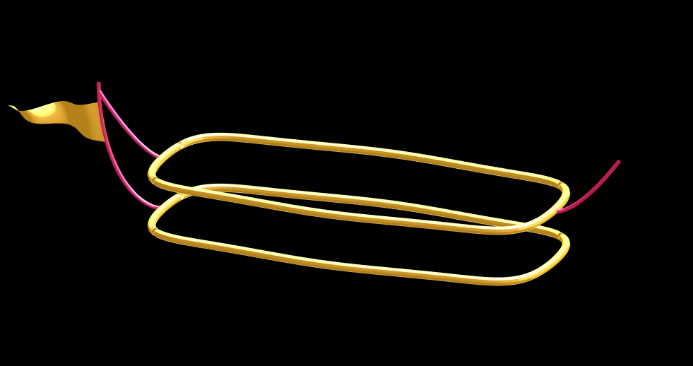
And, very last, we are going to add a flag attached to the outer cable. Let's make it flap in the wind. To make it we will recycle the z3 matrix again, but taper it based on its x-value. Then we will sinusoidally oscillate the flag in the y dimension as a function of x, constraining the y-position to be zero where it meets the cable. Lastly, we will displace it quadratically in the x-dimension as a function of z so that it lines up nicely with the rope. The phase of the sine-function is modified in the animation loop to give it a flapping motion.
h=linspace(0,1);
sc=10;
[fx,fz]=meshgrid(h,h-.5);
F=surf(sc*2.5*fx-90-2*(fz+.5).^2,sc*.3*erf(3*(1-h)).*sin(10*fx+n/5),sc*fz.*h+25,0*fx+c3,'Parent',P);
Plotting just the cables and flag shows:
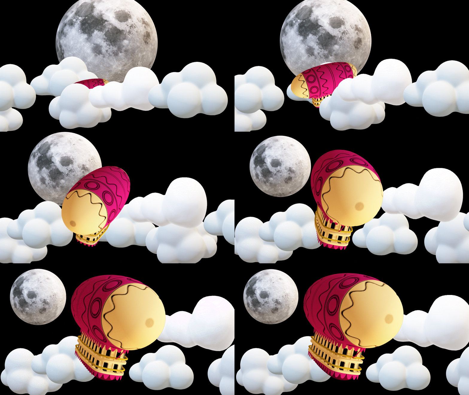
Putting all the pieces together reveals the full airship:
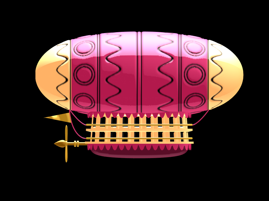
A note about lighting: lighting and material properties really change the feel of the image you create. The above picture is rendered in a cartoony style by setting the specular exponent to a very low value (1), and adding lots of diffuse and ambient reflectivity as well. A light below the airship was also added, albeit with lower strength. Settings used for this plot were:
shading flat
view([0, 0]);
L=light;
L.Color = [1,1,1]/4;
light('position', [0, 0.5, 1], 'color', [1,1,1]);
light('position', [0, 1, -1], 'color', [1, 1, 1]/5);
material([1, 1, .7, 1])
set(gcf, 'color', 'k');
axis equal off
What about all the rest of the stuff (clouds, moon, atmospheric haze etc.) These were all (mostly) recycled bits from previous minihack entries. The clouds were made using power-law noise as explained in Adam Danz' blog post. The moon was borrowed from moonrun, but with an increased number of points. Atmospheric haze was recycled from Matlon5. The rest is just camera angles, hgtransform matrix updates, and updating alpha-maps or vertex coordinates.
Finally, the use of hann() adds the signal processing toolbox as a dependency. To avoid this use the following anonymous function:
hann = @(x)-cospi(linspace(0,2,x)')/2+.5;
16 Comments
Time DescendingTotally awe-inspiring and inspirational Tim, Thank you. You've started a video matlab revolution. ILM would be envious.Excellent story line about "Little Nemo's Airship" as a kid. Mine was "Return to Zork" on a 386sx PC. 5-Stars - Mark Jackson - Cognizant/JetNetSys, LLC
Amazing coding, idea, effects, and overall results!
Compliments! 👏🏻
This is absolutely sensational Tim! You really never cease to amaze us. I had a lot of fun playing around with this. For anyone interested, I have exported the 3d render to .obj and .html formats. Happy to share
Interesting, can we do similar thing here?
This is amazing!! Thanks for sharing.
awsome! wow!
WOW
This is amazing and art of MATLAB.
Thanks for sharing with the community this article.
Wow!
Sign in to participate