Troubleshooting Credit Scorecard Results

This topic shows some of the results when using credit scorecards that need troubleshooting. These examples cover the full range of the credit score card workflow. For details on the overall process of creating and developing credit scorecards, see Credit Scorecard Modeling Workflow.

Predictor Name Is Unspecified and the Parser Returns an Error

If you attempt to use modifybins, bininfo, or plotbins and omit the predictor's name, the parser returns an error.

load CreditCardData
sc = creditscorecard(data,'IDVar','CustID','GoodLabel',0);
modifybins(sc,'CutPoints',[20 30 50 65])

Error using creditscorecard/modifybins (line 79)
Expected a string for the parameter name, instead the input type was 'double'.

Solution: Make sure to include the predictor’s name when using these functions. Use this syntax to specify the PredictorName when using modifybins.

load CreditCardData
sc = creditscorecard(data,'IDVar','CustID','GoodLabel',0);
modifybins(sc,'CustIncome','CutPoints',[20 30 50 65]);

Using bininfo or plotbins Before Binning

If you use bininfo or plotbins before binning, the results might be unusable.

load CreditCardData
sc = creditscorecard(data,'IDVar','CustID','GoodLabel',0);
bininfo(sc,'CustAge')
plotbins(sc,'CustAge')

ans = 

      Bin       Good    Bad     Odds         WOE       InfoValue 
    ________    ____    ___    _______    _________    __________

    '21'          2       1          2    -0.011271    3.1821e-07
    '22'          3       1          3      0.39419    0.00047977
    '23'          1       2        0.5      -1.3976     0.0053002
    '24'          3       4       0.75      -0.9921     0.0062895
    '25'          3       1          3      0.39419    0.00047977
    '26'          4       2          2    -0.011271    6.3641e-07
    '27'          6       5        1.2      -0.5221     0.0026744
    '28'         10       2          5      0.90502     0.0067112
    '29'          8       6     1.3333     -0.41674     0.0021465
    '30'          9      10        0.9     -0.80978      0.011321
    '31'          8       6     1.3333     -0.41674     0.0021465
    '32'         13      13          1     -0.70442      0.011663
    '33'          9      11    0.81818     -0.90509      0.014934
    '34'         14      12     1.1667     -0.55027     0.0070391
    '35'         18      10        1.8     -0.11663    0.00032342
    '36'         23      14     1.6429     -0.20798     0.0013772
    '37'         28      19     1.4737     -0.31665     0.0041132
    '38'         24      14     1.7143     -0.16542     0.0008894
    '39'         21      14        1.5     -0.29895     0.0027242
    '40'         31      12     2.5833      0.24466     0.0020499
    '41'         21      18     1.1667     -0.55027      0.010559
    '42'         29       9     3.2222      0.46565     0.0062605
    '43'         29      23     1.2609     -0.47262      0.010312
    '44'         28      16       1.75      -0.1448    0.00078672
    '45'         36      16       2.25      0.10651    0.00048246
    '46'         33      19     1.7368     -0.15235     0.0010303
    '47'         28       6     4.6667      0.83603      0.016516
    '48'         32      17     1.8824    -0.071896    0.00021357
    '49'         38      10        3.8      0.63058      0.013957
    '50'         33      14     2.3571      0.15303    0.00089239
    '51'         28       9     3.1111      0.43056     0.0052525
    '52'         35       8      4.375      0.77149       0.01808
    '53'         14       8       1.75      -0.1448    0.00039336
    '54'         27      12       2.25      0.10651    0.00036184
    '55'         20       9     2.2222     0.094089    0.00021044
    '56'         20      11     1.8182     -0.10658    0.00029856
    '57'         16       7     2.2857      0.12226    0.00028035
    '58'         11       7     1.5714     -0.25243    0.00099297
    '59'         11       6     1.8333    -0.098283    0.00013904
    '60'          9       4       2.25      0.10651    0.00012061
    '61'         11       2        5.5       1.0003     0.0086637
    '62'          8       0        Inf          Inf           Inf
    '63'          7       1          7       1.2415     0.0076953
    '64'         10       0        Inf          Inf           Inf
    '65'          4       1          4      0.68188     0.0016791
    '66'          6       1          6       1.0873     0.0053857
    '67'          2       3    0.66667      -1.1099     0.0056227
    '68'          6       1          6       1.0873     0.0053857
    '69'          6       0        Inf          Inf           Inf
    '70'          1       0        Inf          Inf           Inf
    '71'          1       0        Inf          Inf           Inf
    '72'          1       0        Inf          Inf           Inf
    '73'          3       0        Inf          Inf           Inf
    '74'          1       0        Inf          Inf           Inf
    'Totals'    803     397     2.0227          NaN           Inf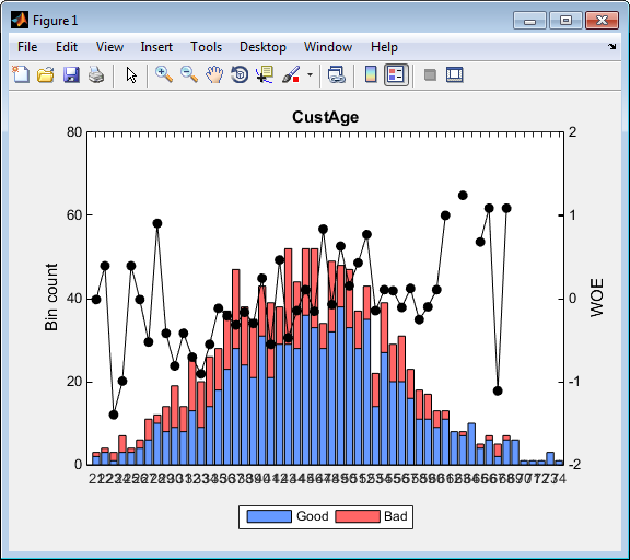

The plot for CustAge is not readable because it has too many bins. Also, bininfo returns data that have Inf values for the WOE due to zero observations for either Good or Bad.

Solution: Bin the data using autobinning or modifybins before plotting or inquiring about the bin statistics, to avoid having too many bins or having NaNs and Infs. For example, you can use the name-value pair argument for AlgoOptions with the autobinning function to define the number of bins.

load CreditCardData
sc = creditscorecard(data,'IDVar','CustID','GoodLabel',0);
AlgoOptions = {'NumBins',4};
sc = autobinning(sc,'CustAge','Algorithm','EqualFrequency',...
'AlgorithmOptions',AlgoOptions);
bininfo(sc,'CustAge','Totals','off')
plotbins(sc,'CustAge')

ans = 

        Bin        Good    Bad     Odds       WOE       InfoValue
    ___________    ____    ___    ______    ________    _________

    '[-Inf,39)'    186     133    1.3985    -0.36902      0.03815
    '[39,46)'      195     108    1.8056    -0.11355    0.0033158
    '[46,52)'      192      75      2.56     0.23559     0.011823
    '[52,Inf]'     230      81    2.8395     0.33921      0.02795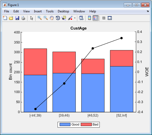

If Categorical Data Is Given as Numeric

Categorical data is often recorded using numeric values, and can be stored in a numeric array. Although you know that the data should be interpreted as categorical information, for creditscorecard this predictor looks like a numeric array.

To show the case where categorical data is given as numeric data, the data for the variable ResStatus is intentionally converted to numeric values.

load CreditCardData
data.ResStatus = double(data.ResStatus);
sc = creditscorecard(data,'IDVar','CustID')

sc = 

  creditscorecard with properties:

                GoodLabel: 0
              ResponseVar: 'status'
                 VarNames: {1x11 cell}
        NumericPredictors: {1x7 cell}
    CategoricalPredictors: {'EmpStatus'  'OtherCC'}
                    IDVar: 'CustID'
            PredictorVars: {1x9 cell}

Note that 'ResStatus' appears as part of the NumericPredictors property. If we applied automatic binning, the resulting bin information raises flags regarding the predictor type.

sc = autobinning(sc,'ResStatus');
[bi,cg] = bininfo(sc,'ResStatus')

bi = 

       Bin        Good    Bad     Odds        WOE       InfoValue 
    __________    ____    ___    ______    _________    __________

    '[-Inf,2)'    365     177    2.0621     0.019329     0.0001682
    '[2,Inf]'     438     220    1.9909    -0.015827    0.00013772
    'Totals'      803     397    2.0227          NaN    0.00030592


cg =

     2

The numeric ranges in the bin labels show that 'ResStatus' is being treated as a numeric variable. This is also confirmed by the fact that the optional output from bininfo is a numeric array of cut points, as opposed to a table with category groupings. Moreover, the output from predictorinfo confirms that the credit scorecard is treating the data as numeric.

[T,Stats] = predictorinfo(sc,'ResStatus')

T = 

                 PredictorType        LatestBinning     
                 _____________    ______________________

    ResStatus    'Numeric'        'Automatic / Monotone'


Stats = 

             Value 
            _______

    Min           1
    Max           3
    Mean     1.7017
    Std     0.71863

Solution: For creditscorecard, 'Categorical' means a MATLAB^® categorical data type. For more information, see categorical. To treat'ResStatus' as categorical, change the 'PredictorType' of the PredictorName 'ResStatus' from 'Numeric' to 'Categorical' using modifypredictor.

sc = modifypredictor(sc,'ResStatus','PredictorType','Categorical')
[T,Stats] = predictorinfo(sc,'ResStatus')

sc = 

  creditscorecard with properties:

                GoodLabel: 0
              ResponseVar: 'status'
                 VarNames: {1x11 cell}
        NumericPredictors: {1x6 cell}
    CategoricalPredictors: {'ResStatus'  'EmpStatus'  'OtherCC'}
                    IDVar: 'CustID'
            PredictorVars: {1x9 cell}


T = 

                 PredictorType    Ordinal     LatestBinning 
                 _____________    _______    _______________

    ResStatus    'Categorical'    false      'Original Data'


Stats = 

          Count
          _____

    C1    542  
    C2    474  
    C3    184  

Note that 'ResStatus' now appears as part of the Categorical predictors. Also, predictorinfo now describes 'ResStatus' as categorical and displays the category counts.

If you apply autobinning, the categories are now reordered, as shown by calling bininfo, which also shows the category labels, as opposed to numeric ranges. The optional output of bininfo is now a category grouping table.

sc = autobinning(sc,'ResStatus');
[bi,cg] = bininfo(sc,'ResStatus')

bi = 

      Bin       Good    Bad     Odds        WOE       InfoValue
    ________    ____    ___    ______    _________    _________

    'C2'        307     167    1.8383    -0.095564    0.0036638
    'C1'        365     177    2.0621     0.019329    0.0001682
    'C3'        131      53    2.4717      0.20049    0.0059418
    'Totals'    803     397    2.0227          NaN    0.0097738


cg = 

    Category    BinNumber
    ________    _________

    'C2'        1        
    'C1'        2        
    'C3'        3        

NaNs Returned When Scoring a “Test” Dataset

When applying a creditscorecard model to a “test” dataset using the score function, if an observation in the “test” dataset has a NaN or <undefined> value, a NaN total score is returned for each of these observations. For example, a creditscorecard object is created using “training” data.

load CreditCardData
sc = creditscorecard(data,'IDVar','CustID');
sc = autobinning(sc);
sc = fitmodel(sc);

1. Adding CustIncome, Deviance = 1490.8527, Chi2Stat = 32.588614, PValue = 1.1387992e-08
2. Adding TmWBank, Deviance = 1467.1415, Chi2Stat = 23.711203, PValue = 1.1192909e-06
3. Adding AMBalance, Deviance = 1455.5715, Chi2Stat = 11.569967, PValue = 0.00067025601
4. Adding EmpStatus, Deviance = 1447.3451, Chi2Stat = 8.2264038, PValue = 0.0041285257
5. Adding CustAge, Deviance = 1441.994, Chi2Stat = 5.3511754, PValue = 0.020708306
6. Adding ResStatus, Deviance = 1437.8756, Chi2Stat = 4.118404, PValue = 0.042419078
7. Adding OtherCC, Deviance = 1433.707, Chi2Stat = 4.1686018, PValue = 0.041179769

Generalized Linear regression model:
    logit(status) ~ 1 + CustAge + ResStatus + EmpStatus + CustIncome + TmWBank + OtherCC + AMBalance
    Distribution = Binomial

Estimated Coefficients:
                   Estimate       SE       tStat       pValue  
                   ________    ________    ______    __________

    (Intercept)    0.70239     0.064001    10.975    5.0538e-28
    CustAge        0.60833      0.24932      2.44      0.014687
    ResStatus        1.377      0.65272    2.1097      0.034888
    EmpStatus      0.88565        0.293    3.0227     0.0025055
    CustIncome     0.70164      0.21844    3.2121     0.0013179
    TmWBank         1.1074      0.23271    4.7589    1.9464e-06
    OtherCC         1.0883      0.52912    2.0569      0.039696
    AMBalance        1.045      0.32214    3.2439     0.0011792


1200 observations, 1192 error degrees of freedom
Dispersion: 1
Chi^2-statistic vs. constant model: 89.7, p-value = 1.4e-16

Suppose that a missing observation (Nan) is added to the data and then newdata is scored using the score function. By default, the points and score assigned to the missing value is NaN.

newdata = data(1:10,:);
newdata.CustAge(1) = NaN;
[Scores,Points] = score(sc,newdata)

Scores =

       NaN
    1.4646
    0.7662
    1.5779
    1.4535
    1.8944
   -0.0872
    0.9207
    1.0399
    0.8252


Points = 

    CustAge     ResStatus    EmpStatus    CustIncome     TmWBank     OtherCC     AMBalance
    ________    _________    _________    __________    _________    ________    _________

         NaN    -0.031252    -0.076317     0.43693        0.39607     0.15842    -0.017472
       0.479      0.12696      0.31449     0.43693      -0.033752     0.15842    -0.017472
     0.21445    -0.031252      0.31449    0.081611        0.39607    -0.19168    -0.017472
     0.23039      0.12696      0.31449     0.43693      -0.044811     0.15842      0.35551
       0.479      0.12696      0.31449     0.43693      -0.044811     0.15842    -0.017472
       0.479      0.12696      0.31449     0.43693        0.39607     0.15842    -0.017472
    -0.14036      0.12696    -0.076317    -0.10466      -0.033752     0.15842    -0.017472
     0.23039      0.37641      0.31449     0.43693      -0.033752    -0.19168     -0.21206
     0.23039    -0.031252    -0.076317     0.43693      -0.033752     0.15842      0.35551
     0.23039      0.12696    -0.076317     0.43693      -0.033752     0.15842    -0.017472

Also, notice that because the CustAge predictor for the first observation is NaN, the corresponding Scores output is NaN also.

Solution: To resolve this issue, use the formatpoints function with the name-value pair argument Missing. When using Missing, you can replace a predictor’s NaN value according to three alternative criteria ('ZeroWoe', 'MinPoints', or 'MaxPoints').

For example, use Missing to replace the missing value with the 'MinPoints' option. The row with the missing data now has a score corresponding to assigning it the minimum possible points for CustAge.

sc = formatpoints(sc,'Missing','MinPoints');
[Scores,Points] = score(sc,newdata)
PointsTable = displaypoints(sc);
PointsTable(1:7,:)

Scores =

    0.7074
    1.4646
    0.7662
    1.5779
    1.4535
    1.8944
   -0.0872
    0.9207
    1.0399
    0.8252


Points = 

    CustAge     ResStatus    EmpStatus    CustIncome     TmWBank     OtherCC     AMBalance
    ________    _________    _________    __________    _________    ________    _________

    -0.15894    -0.031252    -0.076317     0.43693        0.39607     0.15842    -0.017472
       0.479      0.12696      0.31449     0.43693      -0.033752     0.15842    -0.017472
     0.21445    -0.031252      0.31449    0.081611        0.39607    -0.19168    -0.017472
     0.23039      0.12696      0.31449     0.43693      -0.044811     0.15842      0.35551
       0.479      0.12696      0.31449     0.43693      -0.044811     0.15842    -0.017472
       0.479      0.12696      0.31449     0.43693        0.39607     0.15842    -0.017472
    -0.14036      0.12696    -0.076317    -0.10466      -0.033752     0.15842    -0.017472
     0.23039      0.37641      0.31449     0.43693      -0.033752    -0.19168     -0.21206
     0.23039    -0.031252    -0.076317     0.43693      -0.033752     0.15842      0.35551
     0.23039      0.12696    -0.076317     0.43693      -0.033752     0.15842    -0.017472


ans = 

    Predictors        Bin         Points  
    __________    ___________    _________

    'CustAge'     '[-Inf,33)'     -0.15894
    'CustAge'     '[33,37)'       -0.14036
    'CustAge'     '[37,40)'      -0.060323
    'CustAge'     '[40,46)'       0.046408
    'CustAge'     '[46,48)'        0.21445
    'CustAge'     '[48,58)'        0.23039
    'CustAge'     '[58,Inf]'         0.479

Notice that the Scores output has a value for the first customer record because CustAge now has a value and the score can be calculated for the first customer record.