formatpoints
Format scorecard points and scaling
Description
sc = formatpoints(sc,Name,Value)
Examples
This example shows how to use formatpoints to scale by providing the points, odds levels, and PDO (points to double the odds). By using formatpoints to scale, you can put points and scores in a desired range that is more meaningful for practical purposes. Technically, this involves a linear transformation from the unscaled to the scaled points by the formatpoints function.
Create a creditscorecard object using the CreditCardData.mat file to load the data (using a dataset from Refaat 2011). Use the 'IDVar' argument in creditscorecard to indicate that 'CustID' contains ID information and should not be included as a predictor variable.
load CreditCardData
sc = creditscorecard(data,'IDVar','CustID');
Perform automatic binning to bin for all predictors.
sc = autobinning(sc);
Fit a linear regression model using default parameters.
sc = fitmodel(sc);
1. Adding CustIncome, Deviance = 1490.8527, Chi2Stat = 32.588614, PValue = 1.1387992e-08
2. Adding TmWBank, Deviance = 1467.1415, Chi2Stat = 23.711203, PValue = 1.1192909e-06
3. Adding AMBalance, Deviance = 1455.5715, Chi2Stat = 11.569967, PValue = 0.00067025601
4. Adding EmpStatus, Deviance = 1447.3451, Chi2Stat = 8.2264038, PValue = 0.0041285257
5. Adding CustAge, Deviance = 1441.994, Chi2Stat = 5.3511754, PValue = 0.020708306
6. Adding ResStatus, Deviance = 1437.8756, Chi2Stat = 4.118404, PValue = 0.042419078
7. Adding OtherCC, Deviance = 1433.707, Chi2Stat = 4.1686018, PValue = 0.041179769

Generalized linear regression model:
    logit(status) ~ 1 + CustAge + ResStatus + EmpStatus + CustIncome + TmWBank + OtherCC + AMBalance
    Distribution = Binomial

Estimated Coefficients:
                   Estimate       SE       tStat       pValue
                   ________    ________    ______    __________

    (Intercept)    0.70239     0.064001    10.975    5.0538e-28
    CustAge        0.60833      0.24932      2.44      0.014687
    ResStatus        1.377      0.65272    2.1097      0.034888
    EmpStatus      0.88565        0.293    3.0227     0.0025055
    CustIncome     0.70164      0.21844    3.2121     0.0013179
    TmWBank         1.1074      0.23271    4.7589    1.9464e-06
    OtherCC         1.0883      0.52912    2.0569      0.039696
    AMBalance        1.045      0.32214    3.2439     0.0011792


1200 observations, 1192 error degrees of freedom
Dispersion: 1
Chi^2-statistic vs. constant model: 89.7, p-value = 1.4e-16
Display unscaled points for predictors retained in the fitting model and display the minimum and maximum possible unscaled scores.
[PointsInfo,MinScore,MaxScore] = displaypoints(sc)
PointsInfo=37×3 table
      Predictors            Bin            Points
    ______________    ________________    _________

    {'CustAge'   }    {'[-Inf,33)'   }     -0.15894
    {'CustAge'   }    {'[33,37)'     }     -0.14036
    {'CustAge'   }    {'[37,40)'     }    -0.060323
    {'CustAge'   }    {'[40,46)'     }     0.046408
    {'CustAge'   }    {'[46,48)'     }      0.21445
    {'CustAge'   }    {'[48,58)'     }      0.23039
    {'CustAge'   }    {'[58,Inf]'    }        0.479
    {'CustAge'   }    {'<missing>'   }          NaN
    {'ResStatus' }    {'Tenant'      }    -0.031252
    {'ResStatus' }    {'Home Owner'  }      0.12696
    {'ResStatus' }    {'Other'       }      0.37641
    {'ResStatus' }    {'<missing>'   }          NaN
    {'EmpStatus' }    {'Unknown'     }    -0.076317
    {'EmpStatus' }    {'Employed'    }      0.31449
    {'EmpStatus' }    {'<missing>'   }          NaN
    {'CustIncome'}    {'[-Inf,29000)'}     -0.45716
      ⋮
MinScore =
-1.3100
MaxScore =
3.0726
Scale by providing the points, odds levels, and PDO (points to double the odds). Suppose that you want a score of 500 points to have odds of 2 (twice as likely to be good than to be bad) and that the odds double every 50 points (so that 550 points would have odds of 4).
sc = formatpoints(sc,'PointsOddsAndPDO',[500 2 50]);
[PointsInfo,MinScore,MaxScore] = displaypoints(sc)PointsInfo=37×3 table
Predictors Bin Points
______________ ________________ ______
{'CustAge' } {'[-Inf,33)' } 52.821
{'CustAge' } {'[33,37)' } 54.161
{'CustAge' } {'[37,40)' } 59.934
{'CustAge' } {'[40,46)' } 67.633
{'CustAge' } {'[46,48)' } 79.755
{'CustAge' } {'[48,58)' } 80.905
{'CustAge' } {'[58,Inf]' } 98.838
{'CustAge' } {'<missing>' } NaN
{'ResStatus' } {'Tenant' } 62.031
{'ResStatus' } {'Home Owner' } 73.444
{'ResStatus' } {'Other' } 91.438
{'ResStatus' } {'<missing>' } NaN
{'EmpStatus' } {'Unknown' } 58.781
{'EmpStatus' } {'Employed' } 86.971
{'EmpStatus' } {'<missing>' } NaN
{'CustIncome'} {'[-Inf,29000)'} 31.309
⋮
MinScore =
355.5051
MaxScore =
671.6403
This example shows how to use formatpoints to scale by providing the Worst and Best score values. By using formatpoints to scale, you can put points and scores in a desired range that is more meaningful for practical purposes. Technically, this involves a linear transformation from the unscaled to the scaled points.
Create a creditscorecard object using the CreditCardData.mat file to load the data (using a dataset from Refaat 2011). Use the 'IDVar' argument in creditscorecard to indicate that 'CustID' contains ID information and should not be included as a predictor variable.
load CreditCardData
sc = creditscorecard(data,'IDVar','CustID');
Perform automatic binning to bin for all predictors.
sc = autobinning(sc);
Fit a linear regression model using default parameters.
sc = fitmodel(sc);
1. Adding CustIncome, Deviance = 1490.8527, Chi2Stat = 32.588614, PValue = 1.1387992e-08
2. Adding TmWBank, Deviance = 1467.1415, Chi2Stat = 23.711203, PValue = 1.1192909e-06
3. Adding AMBalance, Deviance = 1455.5715, Chi2Stat = 11.569967, PValue = 0.00067025601
4. Adding EmpStatus, Deviance = 1447.3451, Chi2Stat = 8.2264038, PValue = 0.0041285257
5. Adding CustAge, Deviance = 1441.994, Chi2Stat = 5.3511754, PValue = 0.020708306
6. Adding ResStatus, Deviance = 1437.8756, Chi2Stat = 4.118404, PValue = 0.042419078
7. Adding OtherCC, Deviance = 1433.707, Chi2Stat = 4.1686018, PValue = 0.041179769

Generalized linear regression model:
    logit(status) ~ 1 + CustAge + ResStatus + EmpStatus + CustIncome + TmWBank + OtherCC + AMBalance
    Distribution = Binomial

Estimated Coefficients:
                   Estimate       SE       tStat       pValue
                   ________    ________    ______    __________

    (Intercept)    0.70239     0.064001    10.975    5.0538e-28
    CustAge        0.60833      0.24932      2.44      0.014687
    ResStatus        1.377      0.65272    2.1097      0.034888
    EmpStatus      0.88565        0.293    3.0227     0.0025055
    CustIncome     0.70164      0.21844    3.2121     0.0013179
    TmWBank         1.1074      0.23271    4.7589    1.9464e-06
    OtherCC         1.0883      0.52912    2.0569      0.039696
    AMBalance        1.045      0.32214    3.2439     0.0011792


1200 observations, 1192 error degrees of freedom
Dispersion: 1
Chi^2-statistic vs. constant model: 89.7, p-value = 1.4e-16
Display unscaled points for predictors retained in the fitting model and display the minimum and maximum possible unscaled scores.
[PointsInfo,MinScore,MaxScore] = displaypoints(sc)
PointsInfo=37×3 table
      Predictors            Bin            Points
    ______________    ________________    _________

    {'CustAge'   }    {'[-Inf,33)'   }     -0.15894
    {'CustAge'   }    {'[33,37)'     }     -0.14036
    {'CustAge'   }    {'[37,40)'     }    -0.060323
    {'CustAge'   }    {'[40,46)'     }     0.046408
    {'CustAge'   }    {'[46,48)'     }      0.21445
    {'CustAge'   }    {'[48,58)'     }      0.23039
    {'CustAge'   }    {'[58,Inf]'    }        0.479
    {'CustAge'   }    {'<missing>'   }          NaN
    {'ResStatus' }    {'Tenant'      }    -0.031252
    {'ResStatus' }    {'Home Owner'  }      0.12696
    {'ResStatus' }    {'Other'       }      0.37641
    {'ResStatus' }    {'<missing>'   }          NaN
    {'EmpStatus' }    {'Unknown'     }    -0.076317
    {'EmpStatus' }    {'Employed'    }      0.31449
    {'EmpStatus' }    {'<missing>'   }          NaN
    {'CustIncome'}    {'[-Inf,29000)'}     -0.45716
      ⋮
MinScore =
-1.3100
MaxScore =
3.0726
Scale by providing the 'Worst' and 'Best' score values. The range provided below is a common score range. Display the points information again to verify that they are now scaled and also display the scaled minimum and maximum scores.
sc = formatpoints(sc,'WorstAndBestScores',[300 850]);
[PointsInfo,MinScore,MaxScore] = displaypoints(sc)PointsInfo=37×3 table
Predictors Bin Points
______________ ________________ ______
{'CustAge' } {'[-Inf,33)' } 46.396
{'CustAge' } {'[33,37)' } 48.727
{'CustAge' } {'[37,40)' } 58.772
{'CustAge' } {'[40,46)' } 72.167
{'CustAge' } {'[46,48)' } 93.256
{'CustAge' } {'[48,58)' } 95.256
{'CustAge' } {'[58,Inf]' } 126.46
{'CustAge' } {'<missing>' } NaN
{'ResStatus' } {'Tenant' } 62.421
{'ResStatus' } {'Home Owner' } 82.276
{'ResStatus' } {'Other' } 113.58
{'ResStatus' } {'<missing>' } NaN
{'EmpStatus' } {'Unknown' } 56.765
{'EmpStatus' } {'Employed' } 105.81
{'EmpStatus' } {'<missing>' } NaN
{'CustIncome'} {'[-Inf,29000)'} 8.9706
⋮
MinScore =
300.0000
MaxScore =
850.0000
As expected, the values of MinScore and MaxScore correspond to the desired worst and best scores.
This example shows how to use formatpoints to scale by providing the Shift and Slope values. By using formatpoints to scale, you can put points and scores in a desired range that is more meaningful for practical purposes. Technically, this involves a linear transformation from the unscaled to the scaled points by the formatpoints function.
Create a creditscorecard object using the CreditCardData.mat file to load the data (using a dataset from Refaat 2011). Use the 'IDVar' argument in creditscorecard to indicate that 'CustID' contains ID information and should not be included as a predictor variable.
load CreditCardData
sc = creditscorecard(data,'IDVar','CustID');
Perform automatic binning to bin for all predictors.
sc = autobinning(sc);
Fit a linear regression model using default parameters.
sc = fitmodel(sc);
1. Adding CustIncome, Deviance = 1490.8527, Chi2Stat = 32.588614, PValue = 1.1387992e-08
2. Adding TmWBank, Deviance = 1467.1415, Chi2Stat = 23.711203, PValue = 1.1192909e-06
3. Adding AMBalance, Deviance = 1455.5715, Chi2Stat = 11.569967, PValue = 0.00067025601
4. Adding EmpStatus, Deviance = 1447.3451, Chi2Stat = 8.2264038, PValue = 0.0041285257
5. Adding CustAge, Deviance = 1441.994, Chi2Stat = 5.3511754, PValue = 0.020708306
6. Adding ResStatus, Deviance = 1437.8756, Chi2Stat = 4.118404, PValue = 0.042419078
7. Adding OtherCC, Deviance = 1433.707, Chi2Stat = 4.1686018, PValue = 0.041179769

Generalized linear regression model:
    logit(status) ~ 1 + CustAge + ResStatus + EmpStatus + CustIncome + TmWBank + OtherCC + AMBalance
    Distribution = Binomial

Estimated Coefficients:
                   Estimate       SE       tStat       pValue
                   ________    ________    ______    __________

    (Intercept)    0.70239     0.064001    10.975    5.0538e-28
    CustAge        0.60833      0.24932      2.44      0.014687
    ResStatus        1.377      0.65272    2.1097      0.034888
    EmpStatus      0.88565        0.293    3.0227     0.0025055
    CustIncome     0.70164      0.21844    3.2121     0.0013179
    TmWBank         1.1074      0.23271    4.7589    1.9464e-06
    OtherCC         1.0883      0.52912    2.0569      0.039696
    AMBalance        1.045      0.32214    3.2439     0.0011792


1200 observations, 1192 error degrees of freedom
Dispersion: 1
Chi^2-statistic vs. constant model: 89.7, p-value = 1.4e-16
Display unscaled points for predictors retained in the fitting model and display the minimum and maximum possible unscaled scores.
[PointsInfo,MinScore,MaxScore] = displaypoints(sc)
PointsInfo=37×3 table
      Predictors            Bin            Points
    ______________    ________________    _________

    {'CustAge'   }    {'[-Inf,33)'   }     -0.15894
    {'CustAge'   }    {'[33,37)'     }     -0.14036
    {'CustAge'   }    {'[37,40)'     }    -0.060323
    {'CustAge'   }    {'[40,46)'     }     0.046408
    {'CustAge'   }    {'[46,48)'     }      0.21445
    {'CustAge'   }    {'[48,58)'     }      0.23039
    {'CustAge'   }    {'[58,Inf]'    }        0.479
    {'CustAge'   }    {'<missing>'   }          NaN
    {'ResStatus' }    {'Tenant'      }    -0.031252
    {'ResStatus' }    {'Home Owner'  }      0.12696
    {'ResStatus' }    {'Other'       }      0.37641
    {'ResStatus' }    {'<missing>'   }          NaN
    {'EmpStatus' }    {'Unknown'     }    -0.076317
    {'EmpStatus' }    {'Employed'    }      0.31449
    {'EmpStatus' }    {'<missing>'   }          NaN
    {'CustIncome'}    {'[-Inf,29000)'}     -0.45716
      ⋮
MinScore =
-1.3100
MaxScore =
3.0726
Scale by providing the 'Shift' and 'Slope' values. In this example, there is an arbitrary choice of shift and slope. Display the points information again to verify that they are now scaled and also display the scaled minimum and maximum scores.
sc = formatpoints(sc,'ShiftAndSlope',[300 6]);
[PointsInfo,MinScore,MaxScore] = displaypoints(sc)PointsInfo=37×3 table
Predictors Bin Points
______________ ________________ ______
{'CustAge' } {'[-Inf,33)' } 41.904
{'CustAge' } {'[33,37)' } 42.015
{'CustAge' } {'[37,40)' } 42.495
{'CustAge' } {'[40,46)' } 43.136
{'CustAge' } {'[46,48)' } 44.144
{'CustAge' } {'[48,58)' } 44.239
{'CustAge' } {'[58,Inf]' } 45.731
{'CustAge' } {'<missing>' } NaN
{'ResStatus' } {'Tenant' } 42.67
{'ResStatus' } {'Home Owner' } 43.619
{'ResStatus' } {'Other' } 45.116
{'ResStatus' } {'<missing>' } NaN
{'EmpStatus' } {'Unknown' } 42.399
{'EmpStatus' } {'Employed' } 44.744
{'EmpStatus' } {'<missing>' } NaN
{'CustIncome'} {'[-Inf,29000)'} 40.114
⋮
MinScore =
292.1401
MaxScore =
318.4355
This example shows how to use formatpoints to separate the base points from the rest of the points assigned to each predictor variable. The formatpoints name-value pair argument 'BasePoints' serves this purpose.
Create a creditscorecard object using the CreditCardData.mat file to load the data (using a dataset from Refaat 2011). Use the 'IDVar' argument in creditscorecard to indicate that 'CustID' contains ID information and should not be included as a predictor variable.
load CreditCardData
sc = creditscorecard(data,'IDVar','CustID');
Perform automatic binning to bin for all predictors.
sc = autobinning(sc);
Fit a linear regression model using default parameters.
sc = fitmodel(sc);
1. Adding CustIncome, Deviance = 1490.8527, Chi2Stat = 32.588614, PValue = 1.1387992e-08
2. Adding TmWBank, Deviance = 1467.1415, Chi2Stat = 23.711203, PValue = 1.1192909e-06
3. Adding AMBalance, Deviance = 1455.5715, Chi2Stat = 11.569967, PValue = 0.00067025601
4. Adding EmpStatus, Deviance = 1447.3451, Chi2Stat = 8.2264038, PValue = 0.0041285257
5. Adding CustAge, Deviance = 1441.994, Chi2Stat = 5.3511754, PValue = 0.020708306
6. Adding ResStatus, Deviance = 1437.8756, Chi2Stat = 4.118404, PValue = 0.042419078
7. Adding OtherCC, Deviance = 1433.707, Chi2Stat = 4.1686018, PValue = 0.041179769

Generalized linear regression model:
    logit(status) ~ 1 + CustAge + ResStatus + EmpStatus + CustIncome + TmWBank + OtherCC + AMBalance
    Distribution = Binomial

Estimated Coefficients:
                   Estimate       SE       tStat       pValue
                   ________    ________    ______    __________

    (Intercept)    0.70239     0.064001    10.975    5.0538e-28
    CustAge        0.60833      0.24932      2.44      0.014687
    ResStatus        1.377      0.65272    2.1097      0.034888
    EmpStatus      0.88565        0.293    3.0227     0.0025055
    CustIncome     0.70164      0.21844    3.2121     0.0013179
    TmWBank         1.1074      0.23271    4.7589    1.9464e-06
    OtherCC         1.0883      0.52912    2.0569      0.039696
    AMBalance        1.045      0.32214    3.2439     0.0011792


1200 observations, 1192 error degrees of freedom
Dispersion: 1
Chi^2-statistic vs. constant model: 89.7, p-value = 1.4e-16
Display unscaled points for predictors retained in the fitting model and display the minimum and maximum possible unscaled scores.
[PointsInfo,MinScore,MaxScore] = displaypoints(sc)
PointsInfo=37×3 table
      Predictors            Bin            Points
    ______________    ________________    _________

    {'CustAge'   }    {'[-Inf,33)'   }     -0.15894
    {'CustAge'   }    {'[33,37)'     }     -0.14036
    {'CustAge'   }    {'[37,40)'     }    -0.060323
    {'CustAge'   }    {'[40,46)'     }     0.046408
    {'CustAge'   }    {'[46,48)'     }      0.21445
    {'CustAge'   }    {'[48,58)'     }      0.23039
    {'CustAge'   }    {'[58,Inf]'    }        0.479
    {'CustAge'   }    {'<missing>'   }          NaN
    {'ResStatus' }    {'Tenant'      }    -0.031252
    {'ResStatus' }    {'Home Owner'  }      0.12696
    {'ResStatus' }    {'Other'       }      0.37641
    {'ResStatus' }    {'<missing>'   }          NaN
    {'EmpStatus' }    {'Unknown'     }    -0.076317
    {'EmpStatus' }    {'Employed'    }      0.31449
    {'EmpStatus' }    {'<missing>'   }          NaN
    {'CustIncome'}    {'[-Inf,29000)'}     -0.45716
      ⋮
MinScore =
-1.3100
MaxScore =
3.0726
By setting the name-value pair argument BasePoints to true, the points information table reports the base points separately in the first row. The minimum and maximum possible scores are not affected by this option.
sc = formatpoints(sc,'BasePoints',true);
[PointsInfo,MinScore,MaxScore] = displaypoints(sc)PointsInfo=38×3 table
Predictors Bin Points
______________ ______________ _________
{'BasePoints'} {'BasePoints'} 0.70239
{'CustAge' } {'[-Inf,33)' } -0.25928
{'CustAge' } {'[33,37)' } -0.24071
{'CustAge' } {'[37,40)' } -0.16066
{'CustAge' } {'[40,46)' } -0.053933
{'CustAge' } {'[46,48)' } 0.11411
{'CustAge' } {'[48,58)' } 0.13005
{'CustAge' } {'[58,Inf]' } 0.37866
{'CustAge' } {'<missing>' } NaN
{'ResStatus' } {'Tenant' } -0.13159
{'ResStatus' } {'Home Owner'} 0.026616
{'ResStatus' } {'Other' } 0.27607
{'ResStatus' } {'<missing>' } NaN
{'EmpStatus' } {'Unknown' } -0.17666
{'EmpStatus' } {'Employed' } 0.21415
{'EmpStatus' } {'<missing>' } NaN
⋮
MinScore =
-1.3100
MaxScore =
3.0726
This example shows how to use formatpoints to round points. Rounding is usually applied after scaling, otherwise, if the points for a particular predictor are all in a small range, rounding could cause the rounded points for different bins to be the same. Also, rounding all the points may slightly change the minimum and maximum total points.
Create a creditscorecard object using the CreditCardData.mat file to load the data (using a dataset from Refaat 2011). Use the 'IDVar' argument in creditscorecard to indicate that 'CustID' contains ID information and should not be included as a predictor variable.
load CreditCardData
sc = creditscorecard(data,'IDVar','CustID');
Perform automatic binning to bin for all predictors.
sc = autobinning(sc);
Fit a linear regression model using default parameters.
sc = fitmodel(sc);
1. Adding CustIncome, Deviance = 1490.8527, Chi2Stat = 32.588614, PValue = 1.1387992e-08
2. Adding TmWBank, Deviance = 1467.1415, Chi2Stat = 23.711203, PValue = 1.1192909e-06
3. Adding AMBalance, Deviance = 1455.5715, Chi2Stat = 11.569967, PValue = 0.00067025601
4. Adding EmpStatus, Deviance = 1447.3451, Chi2Stat = 8.2264038, PValue = 0.0041285257
5. Adding CustAge, Deviance = 1441.994, Chi2Stat = 5.3511754, PValue = 0.020708306
6. Adding ResStatus, Deviance = 1437.8756, Chi2Stat = 4.118404, PValue = 0.042419078
7. Adding OtherCC, Deviance = 1433.707, Chi2Stat = 4.1686018, PValue = 0.041179769

Generalized linear regression model:
    logit(status) ~ 1 + CustAge + ResStatus + EmpStatus + CustIncome + TmWBank + OtherCC + AMBalance
    Distribution = Binomial

Estimated Coefficients:
                   Estimate       SE       tStat       pValue
                   ________    ________    ______    __________

    (Intercept)    0.70239     0.064001    10.975    5.0538e-28
    CustAge        0.60833      0.24932      2.44      0.014687
    ResStatus        1.377      0.65272    2.1097      0.034888
    EmpStatus      0.88565        0.293    3.0227     0.0025055
    CustIncome     0.70164      0.21844    3.2121     0.0013179
    TmWBank         1.1074      0.23271    4.7589    1.9464e-06
    OtherCC         1.0883      0.52912    2.0569      0.039696
    AMBalance        1.045      0.32214    3.2439     0.0011792


1200 observations, 1192 error degrees of freedom
Dispersion: 1
Chi^2-statistic vs. constant model: 89.7, p-value = 1.4e-16
Display unscaled points for predictors retained in the fitting model and display the minimum and maximum possible unscaled scores.
[PointsInfo,MinScore,MaxScore] = displaypoints(sc)
PointsInfo=37×3 table
      Predictors            Bin            Points
    ______________    ________________    _________

    {'CustAge'   }    {'[-Inf,33)'   }     -0.15894
    {'CustAge'   }    {'[33,37)'     }     -0.14036
    {'CustAge'   }    {'[37,40)'     }    -0.060323
    {'CustAge'   }    {'[40,46)'     }     0.046408
    {'CustAge'   }    {'[46,48)'     }      0.21445
    {'CustAge'   }    {'[48,58)'     }      0.23039
    {'CustAge'   }    {'[58,Inf]'    }        0.479
    {'CustAge'   }    {'<missing>'   }          NaN
    {'ResStatus' }    {'Tenant'      }    -0.031252
    {'ResStatus' }    {'Home Owner'  }      0.12696
    {'ResStatus' }    {'Other'       }      0.37641
    {'ResStatus' }    {'<missing>'   }          NaN
    {'EmpStatus' }    {'Unknown'     }    -0.076317
    {'EmpStatus' }    {'Employed'    }      0.31449
    {'EmpStatus' }    {'<missing>'   }          NaN
    {'CustIncome'}    {'[-Inf,29000)'}     -0.45716
      ⋮
MinScore =
-1.3100
MaxScore =
3.0726
Scale points, and display the points information. By default, no rounding is applied.
sc = formatpoints(sc,'WorstAndBestScores',[300 850]);
PointsInfo = displaypoints(sc)PointsInfo=37×3 table
Predictors Bin Points
______________ ________________ ______
{'CustAge' } {'[-Inf,33)' } 46.396
{'CustAge' } {'[33,37)' } 48.727
{'CustAge' } {'[37,40)' } 58.772
{'CustAge' } {'[40,46)' } 72.167
{'CustAge' } {'[46,48)' } 93.256
{'CustAge' } {'[48,58)' } 95.256
{'CustAge' } {'[58,Inf]' } 126.46
{'CustAge' } {'<missing>' } NaN
{'ResStatus' } {'Tenant' } 62.421
{'ResStatus' } {'Home Owner' } 82.276
{'ResStatus' } {'Other' } 113.58
{'ResStatus' } {'<missing>' } NaN
{'EmpStatus' } {'Unknown' } 56.765
{'EmpStatus' } {'Employed' } 105.81
{'EmpStatus' } {'<missing>' } NaN
{'CustIncome'} {'[-Inf,29000)'} 8.9706
⋮
Use the name-value pair argument Round to apply rounding for all points and then display the points information again.
sc = formatpoints(sc,'Round','AllPoints');
PointsInfo = displaypoints(sc)
PointsInfo=37×3 table
      Predictors            Bin           Points
    ______________    ________________    ______

    {'CustAge'   }    {'[-Inf,33)'   }      46
    {'CustAge'   }    {'[33,37)'     }      49
    {'CustAge'   }    {'[37,40)'     }      59
    {'CustAge'   }    {'[40,46)'     }      72
    {'CustAge'   }    {'[46,48)'     }      93
    {'CustAge'   }    {'[48,58)'     }      95
    {'CustAge'   }    {'[58,Inf]'    }     126
    {'CustAge'   }    {'<missing>'   }     NaN
    {'ResStatus' }    {'Tenant'      }      62
    {'ResStatus' }    {'Home Owner'  }      82
    {'ResStatus' }    {'Other'       }     114
    {'ResStatus' }    {'<missing>'   }     NaN
    {'EmpStatus' }    {'Unknown'     }      57
    {'EmpStatus' }    {'Employed'    }     106
    {'EmpStatus' }    {'<missing>'   }     NaN
    {'CustIncome'}    {'[-Inf,29000)'}       9
      ⋮
This example shows that rounding scorecard points can modify the original risk ranking of a credit scorecard. You can control rounding by using formatpoints with the optional name-value pair argument for 'Rounding'.
Credit scores rank customers by risk. If higher scores are given to better, less risky customers, then higher scores must correspond to lower default probabilities. When you use the name-value pair argument for 'Rounding', depending on the value for 'Rounding', the rounding behavior is:
When
'Rounding'is set to'None'(default option), no rounding is applied to points or scores, and the risk ranking is completely consistent with the calibrated model.When
'Rounding'is set to'FinalScore', rounding is only applied to the final scores. In this case: a) Customers with different scores (different risk) may have the same rounded score. b) Customers with the same rounded score may have different default probabilities. c) Customer with higher rounded scores will always have lower default probability than customers with lower scores.When
'Rounding'is set to'AllPoints', rounding is applied to all points in the scorecard (all bins, all predictors). In this case: a) Customers with different scores (different risk) may have the same rounded score, or their ranking may even be reversed (the customer with the lower original score may have a higher rounded score). b) Customers with the same rounded score may have different default probabilities. c) Customer with higher rounded scores may in some cases have higher default probabilities than customers with lower scores.
Create a creditscorecard
To demonstrate the rounding behavior, first create a creditscorecard object.
load CreditCardData
sc = creditscorecard(data,'IDVar','CustID','ResponseVar','status');
sc = autobinning(sc);
sc = modifybins(sc,'CustIncome','CutPoints',20000:5000:60000);
sc = fitmodel(sc);
1. Adding CustIncome, Deviance = 1487.9719, Chi2Stat = 35.469392, PValue = 2.5909009e-09
2. Adding TmWBank, Deviance = 1465.7998, Chi2Stat = 22.172089, PValue = 2.4927133e-06
3. Adding AMBalance, Deviance = 1455.206, Chi2Stat = 10.593833, PValue = 0.0011346548
4. Adding EmpStatus, Deviance = 1446.3918, Chi2Stat = 8.8142314, PValue = 0.0029889009
5. Adding CustAge, Deviance = 1440.6825, Chi2Stat = 5.709236, PValue = 0.016875883
6. Adding ResStatus, Deviance = 1436.1363, Chi2Stat = 4.5462043, PValue = 0.032991806
7. Adding OtherCC, Deviance = 1431.9546, Chi2Stat = 4.1817827, PValue = 0.040860699

Generalized linear regression model:
    logit(status) ~ 1 + CustAge + ResStatus + EmpStatus + CustIncome + TmWBank + OtherCC + AMBalance
    Distribution = Binomial

Estimated Coefficients:
                   Estimate       SE       tStat       pValue
                   ________    ________    ______    __________

    (Intercept)    0.70247     0.064046    10.968    5.4345e-28
    CustAge        0.60579      0.24405    2.4822      0.013058
    ResStatus       1.4463      0.65427    2.2105       0.02707
    EmpStatus      0.90501      0.29262    3.0928     0.0019828
    CustIncome     0.70869      0.20535    3.4512    0.00055815
    TmWBank         1.0839      0.23244    4.6631    3.1145e-06
    OtherCC         1.0906      0.52936    2.0602      0.039377
    AMBalance       1.0148      0.32273    3.1445     0.0016636


1200 observations, 1192 error degrees of freedom
Dispersion: 1
Chi^2-statistic vs. constant model: 91.5, p-value = 6.12e-17
Apply the 'Rounding' Options
Apply each of the three 'Rounding' options to the creditscorecard object.
sc = formatpoints(sc,'PointsOddsAndPDO',[500 2 50]); % No Rounding
points1  = displaypoints(sc);
[S1,P1]  = score(sc);
defProb1 = probdefault(sc);

sc = formatpoints(sc,'Round','AllPoints'); % 'AllPoints' Rounding
points2  = displaypoints(sc);
[S2,P2]  = score(sc);
defProb2 = probdefault(sc);

sc = formatpoints(sc,'Round','FinalScore'); % 'FinalScore' Rounding
points3  = displaypoints(sc);
[S3,P3]  = score(sc);
defProb3 = probdefault(sc);
Compare the 'Rounding' Options
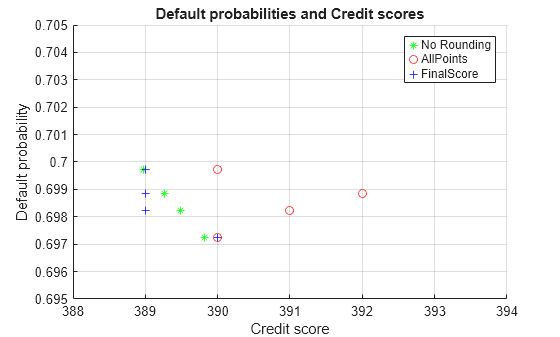
Visualize the default probabilities versus the scores.
figure
hold on
scatter(S1, defProb1, 'g*')
scatter(S2, defProb2, 'ro')
scatter(S3, defProb3, 'b+')
legend('No Rounding','AllPoints','FinalScore')
axis([388 394 0.695 0.705])
xlabel('Credit score')
ylabel('Default probability')
title('Default probabilities and Credit scores')
grid
Inspect the points and total scores for each 'Rounding' option, in table format.
ind = [208 363 694 886];
ProbDefault = defProb1(ind)
ProbDefault = 4×1

    0.6997
    0.6989
    0.6982
    0.6972
% ScoreNoRounding = S1(ind)
PointsNoRounding = P1(ind,:);
PointsNoRounding.Total = S1(ind)PointsNoRounding=4×8 table
CustAge ResStatus EmpStatus CustIncome TmWBank OtherCC AMBalance Total
_______ _________ _________ __________ _______ _______ _________ ______
52.9 61.555 58.503 24.647 51.551 50.416 89.4 388.97
67.65 61.555 58.503 24.647 51.551 75.723 49.64 389.27
54.234 61.555 58.503 24.647 51.551 75.723 63.271 389.48
52.9 92.441 58.503 24.647 61.277 50.416 49.64 389.82
% ScoreAllPoints = S2(ind)
PointsAllPoints = P2(ind,:);
PointsAllPoints.Total = S2(ind)PointsAllPoints=4×8 table
CustAge ResStatus EmpStatus CustIncome TmWBank OtherCC AMBalance Total
_______ _________ _________ __________ _______ _______ _________ _____
53 62 59 25 52 50 89 390
68 62 59 25 52 76 50 392
54 62 59 25 52 76 63 391
53 92 59 25 61 50 50 390
% ScoreFinalScore = S3(ind)
PointsFinalScore = P3(ind,:);
PointsFinalScore.Total = S3(ind)PointsFinalScore=4×8 table
CustAge ResStatus EmpStatus CustIncome TmWBank OtherCC AMBalance Total
_______ _________ _________ __________ _______ _______ _________ _____
52.9 61.555 58.503 24.647 51.551 50.416 89.4 389
67.65 61.555 58.503 24.647 51.551 75.723 49.64 389
54.234 61.555 58.503 24.647 51.551 75.723 63.271 389
52.9 92.441 58.503 24.647 61.277 50.416 49.64 390
The original creditscorecard model, without rounding, was calibrated to the data with a logistic regression. The ranking and probabilities have a statistical foundation.
Rounding, however, effectively modifies the creditscorecard model. When only the final score is rounded, this leads to some "ties" in rounded scores, but at least the risk ranking across scores is preserved (because if s1 <= s2, then round(s1) <= round(s2)).
However, when you round all points, a score may gain extra points by chance. For example, in the second row in the table (row 363 of original data), the points for all predictors are rounded up by almost 0.5. The original score is 389.27. Rounding the final score makes it 389. However, rounding all points makes it 392, that is three points higher than rounding the final score.
This example shows how to use formatpoints to score missing or out-of-range data. When data is scored, some observations can be either missing (NaN, or undefined) or out of range. You will need to decide whether or not points are assigned to these cases. Use the name-value pair argument Missing to do so.
Create a creditscorecard object using the CreditCardData.mat file to load the data (using a dataset from Refaat 2011). Use the 'IDVar' argument in creditscorecard to indicate that 'CustID' contains ID information and should not be included as a predictor variable.
load CreditCardData
sc = creditscorecard(data,'IDVar','CustID');
Perform automatic binning to bin for all predictors.
sc = autobinning(sc);
Indicate that the minimum allowed value for 'CustAge' is zero. This makes any negative values for age invalid or out-of-range.
sc = modifybins(sc,'CustAge','MinValue',0);
Fit a linear regression model using default parameters.
sc = fitmodel(sc);
1. Adding CustIncome, Deviance = 1490.8527, Chi2Stat = 32.588614, PValue = 1.1387992e-08
2. Adding TmWBank, Deviance = 1467.1415, Chi2Stat = 23.711203, PValue = 1.1192909e-06
3. Adding AMBalance, Deviance = 1455.5715, Chi2Stat = 11.569967, PValue = 0.00067025601
4. Adding EmpStatus, Deviance = 1447.3451, Chi2Stat = 8.2264038, PValue = 0.0041285257
5. Adding CustAge, Deviance = 1441.994, Chi2Stat = 5.3511754, PValue = 0.020708306
6. Adding ResStatus, Deviance = 1437.8756, Chi2Stat = 4.118404, PValue = 0.042419078
7. Adding OtherCC, Deviance = 1433.707, Chi2Stat = 4.1686018, PValue = 0.041179769

Generalized linear regression model:
    logit(status) ~ 1 + CustAge + ResStatus + EmpStatus + CustIncome + TmWBank + OtherCC + AMBalance
    Distribution = Binomial

Estimated Coefficients:
                   Estimate       SE       tStat       pValue
                   ________    ________    ______    __________

    (Intercept)    0.70239     0.064001    10.975    5.0538e-28
    CustAge        0.60833      0.24932      2.44      0.014687
    ResStatus        1.377      0.65272    2.1097      0.034888
    EmpStatus      0.88565        0.293    3.0227     0.0025055
    CustIncome     0.70164      0.21844    3.2121     0.0013179
    TmWBank         1.1074      0.23271    4.7589    1.9464e-06
    OtherCC         1.0883      0.52912    2.0569      0.039696
    AMBalance        1.045      0.32214    3.2439     0.0011792


1200 observations, 1192 error degrees of freedom
Dispersion: 1
Chi^2-statistic vs. constant model: 89.7, p-value = 1.4e-16
Suppose there are missing or out of range observations in the data that you want to score. Notice that by default, the points and score assigned to the missing value is NaN.
% Set up a data set with missing and out of range data for illustration purposes
newdata = data(1:5,:);
newdata.CustAge(1) = NaN; % missing
newdata.CustAge(2) = -100; % invalid
newdata.ResStatus(3) = missing; % missing
newdata.ResStatus(4) = 'House'; % invalid
disp(newdata)
    CustID    CustAge    TmAtAddress     ResStatus     EmpStatus    CustIncome    TmWBank    OtherCC    AMBalance    UtilRate    status
    ______    _______    ___________    ___________    _________    __________    _______    _______    _________    ________    ______

      1         NaN          62         Tenant         Unknown        50000         55         Yes       1055.9        0.22        0
      2        -100          22         Home Owner     Employed       52000         25         Yes       1161.6        0.24        0
      3          47          30         <undefined>    Employed       37000         61         No        877.23        0.29        0
      4          50          75         House          Employed       53000         20         Yes       157.37        0.08        0
      5          68          56         Home Owner     Employed       53000         14         Yes       561.84        0.11        0
[Scores,Points] = score(sc,newdata);
disp(Scores)
       NaN
       NaN
       NaN
       NaN
    1.4535
disp(Points)
    CustAge    ResStatus    EmpStatus    CustIncome     TmWBank     OtherCC     AMBalance
    _______    _________    _________    __________    _________    ________    _________

        NaN    -0.031252    -0.076317      0.43693       0.39607     0.15842    -0.017472
        NaN      0.12696      0.31449      0.43693     -0.033752     0.15842    -0.017472
    0.21445          NaN      0.31449     0.081611       0.39607    -0.19168    -0.017472
    0.23039          NaN      0.31449      0.43693     -0.044811     0.15842      0.35551
      0.479      0.12696      0.31449      0.43693     -0.044811     0.15842    -0.017472
Use the name-value pair argument Missing to replace NaN with points corresponding to a zero Weight-of-Evidence (WOE).
sc = formatpoints(sc,'Missing','ZeroWOE');
[Scores,Points] = score(sc,newdata);
disp(Scores)
    0.9667
    1.0859
    0.8978
    1.5513
    1.4535
disp(Points)
    CustAge    ResStatus    EmpStatus    CustIncome     TmWBank     OtherCC     AMBalance
    _______    _________    _________    __________    _________    ________    _________

    0.10034    -0.031252    -0.076317      0.43693       0.39607     0.15842    -0.017472
    0.10034      0.12696      0.31449      0.43693     -0.033752     0.15842    -0.017472
    0.21445      0.10034      0.31449     0.081611       0.39607    -0.19168    -0.017472
    0.23039      0.10034      0.31449      0.43693     -0.044811     0.15842      0.35551
      0.479      0.12696      0.31449      0.43693     -0.044811     0.15842    -0.017472
Alternatively, use the name-value pair argument Missing to replace the missing value with the minimum points for the predictors that have the missing values.
sc = formatpoints(sc,'Missing','MinPoints');
[Scores,Points] = score(sc,newdata);
disp(Scores)
    0.7074
    0.8266
    0.7662
    1.4197
    1.4535
disp(Points)
    CustAge     ResStatus    EmpStatus    CustIncome     TmWBank     OtherCC     AMBalance
    ________    _________    _________    __________    _________    ________    _________

    -0.15894    -0.031252    -0.076317      0.43693       0.39607     0.15842    -0.017472
    -0.15894      0.12696      0.31449      0.43693     -0.033752     0.15842    -0.017472
     0.21445    -0.031252      0.31449     0.081611       0.39607    -0.19168    -0.017472
     0.23039    -0.031252      0.31449      0.43693     -0.044811     0.15842      0.35551
       0.479      0.12696      0.31449      0.43693     -0.044811     0.15842    -0.017472
As a third alternative, use the name-value pair argument Missing to replace the missing value with the maximum points for the predictors that have the missing values.
sc = formatpoints(sc,'Missing','MaxPoints');
[Scores,Points] = score(sc,newdata);
disp(Scores)
    1.3454
    1.4646
    1.1739
    1.8273
    1.4535
disp(Points)
    CustAge    ResStatus    EmpStatus    CustIncome     TmWBank     OtherCC     AMBalance
    _______    _________    _________    __________    _________    ________    _________

      0.479    -0.031252    -0.076317      0.43693       0.39607     0.15842    -0.017472
      0.479      0.12696      0.31449      0.43693     -0.033752     0.15842    -0.017472
    0.21445      0.37641      0.31449     0.081611       0.39607    -0.19168    -0.017472
    0.23039      0.37641      0.31449      0.43693     -0.044811     0.15842      0.35551
      0.479      0.12696      0.31449      0.43693     -0.044811     0.15842    -0.017472
Verify that the minimum and maximum points assigned to the missing data correspond to the minimum and maximum points for the corresponding predictors. The points for 'CustAge' are reported in the first seven rows of the points information table. For 'ResStatus' the points are in rows 8 through 10.
PointsInfo = displaypoints(sc);
PointsInfo(1:7,:)
ans=7×3 table
    Predictors         Bin          Points
    ___________    ____________    _________

    {'CustAge'}    {'[0,33)'  }     -0.15894
    {'CustAge'}    {'[33,37)' }     -0.14036
    {'CustAge'}    {'[37,40)' }    -0.060323
    {'CustAge'}    {'[40,46)' }     0.046408
    {'CustAge'}    {'[46,48)' }      0.21445
    {'CustAge'}    {'[48,58)' }      0.23039
    {'CustAge'}    {'[58,Inf]'}        0.479
min(PointsInfo.Points(1:7))
ans =
-0.1589
max(PointsInfo.Points(1:7))
ans =
0.4790
PointsInfo(8:10,:)
ans=3×3 table
     Predictors           Bin           Points
    _____________    ______________    _________

    {'CustAge'  }    {'<missing>' }        0.479
    {'ResStatus'}    {'Tenant'    }    -0.031252
    {'ResStatus'}    {'Home Owner'}      0.12696
min(PointsInfo.Points(8:10))
ans =
-0.0313
max(PointsInfo.Points(8:10))
ans =
0.4790
This example describes the assignment of points for missing data when the 'BinMissingData' option is set to true.
Predictors that have missing data in the training set have an explicit bin for
<missing>with corresponding points in the final scorecard. These points are computed from the Weight-of-Evidence (WOE) value for the<missing>bin and the logistic model coefficients. For scoring purposes, these points are assigned to missing values and to out-of-range values.Predictors with no missing data in the training set have no
<missing>bin, therefore no WOE can be estimated from the training data. By default, the points for missing and out-of-range values are set toNaN, and this leads to a score ofNaNwhen runningscore. For predictors that have no explicit<missing>bin, use the name-value argument'Missing'informatpointsto indicate how missing data should be treated for scoring purposes.
Create a creditscorecard object using the CreditCardData.mat file to load the dataMissing with missing values.
load CreditCardData.mat
head(dataMissing,5)
CustID CustAge TmAtAddress ResStatus EmpStatus CustIncome TmWBank OtherCC AMBalance UtilRate status
______ _______ ___________ ___________ _________ __________ _______ _______ _________ ________ ______
1 53 62 <undefined> Unknown 50000 55 Yes 1055.9 0.22 0
2 61 22 Home Owner Employed 52000 25 Yes 1161.6 0.24 0
3 47 30 Tenant Employed 37000 61 No 877.23 0.29 0
4 NaN 75 Home Owner Employed 53000 20 Yes 157.37 0.08 0
5 68 56 Home Owner Employed 53000 14 Yes 561.84 0.11 0
fprintf('Number of rows: %d\n',height(dataMissing))Number of rows: 1200
fprintf('Number of missing values CustAge: %d\n',sum(ismissing(dataMissing.CustAge)))Number of missing values CustAge: 30
fprintf('Number of missing values ResStatus: %d\n',sum(ismissing(dataMissing.ResStatus)))Number of missing values ResStatus: 40
Use creditscorecard with the name-value argument 'BinMissingData' set to true to bin the missing numeric or categorical data in a separate bin. Apply automatic binning.
sc = creditscorecard(dataMissing,'IDVar','CustID','BinMissingData',true);
sc = autobinning(sc);

disp(sc)
  creditscorecard with properties:

                GoodLabel: 0
              ResponseVar: 'status'
               WeightsVar: ''
                 VarNames: {'CustID'  'CustAge'  'TmAtAddress'  'ResStatus'  'EmpStatus'  'CustIncome'  'TmWBank'  'OtherCC'  'AMBalance'  'UtilRate'  'status'}
        NumericPredictors: {'CustAge'  'TmAtAddress'  'CustIncome'  'TmWBank'  'AMBalance'  'UtilRate'}
    CategoricalPredictors: {'ResStatus'  'EmpStatus'  'OtherCC'}
           BinMissingData: 1
                    IDVar: 'CustID'
            PredictorVars: {'CustAge'  'TmAtAddress'  'ResStatus'  'EmpStatus'  'CustIncome'  'TmWBank'  'OtherCC'  'AMBalance'  'UtilRate'}
                     Data: [1200×11 table]
Set a minimum value of zero for CustAge and CustIncome. With this, any negative age or income information becomes invalid or "out-of-range". For scoring purposes, out-of-range values are given the same points as missing values.
sc = modifybins(sc,'CustAge','MinValue',0);
sc = modifybins(sc,'CustIncome','MinValue',0);
Display and plot bin information for numeric data for 'CustAge' that includes missing data in a separate bin labelled <missing>.
[bi,cp] = bininfo(sc,'CustAge');
disp(bi)
Bin Good Bad Odds WOE InfoValue
_____________ ____ ___ ______ ________ __________
{'[0,33)' } 69 52 1.3269 -0.42156 0.018993
{'[33,37)' } 63 45 1.4 -0.36795 0.012839
{'[37,40)' } 72 47 1.5319 -0.2779 0.0079824
{'[40,46)' } 172 89 1.9326 -0.04556 0.0004549
{'[46,48)' } 59 25 2.36 0.15424 0.0016199
{'[48,51)' } 99 41 2.4146 0.17713 0.0035449
{'[51,58)' } 157 62 2.5323 0.22469 0.0088407
{'[58,Inf]' } 93 25 3.72 0.60931 0.032198
{'<missing>'} 19 11 1.7273 -0.15787 0.00063885
{'Totals' } 803 397 2.0227 NaN 0.087112
plotbins(sc,'CustAge')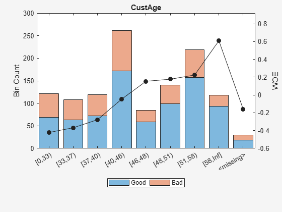
Display and plot bin information for categorical data for 'ResStatus' that includes missing data in a separate bin labelled <missing>.
[bi,cg] = bininfo(sc,'ResStatus');
disp(bi)
Bin Good Bad Odds WOE InfoValue
______________ ____ ___ ______ _________ __________
{'Tenant' } 296 161 1.8385 -0.095463 0.0035249
{'Home Owner'} 352 171 2.0585 0.017549 0.00013382
{'Other' } 128 52 2.4615 0.19637 0.0055808
{'<missing>' } 27 13 2.0769 0.026469 2.3248e-05
{'Totals' } 803 397 2.0227 NaN 0.0092627
plotbins(sc,'ResStatus')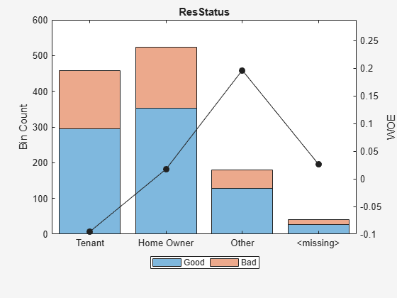
For the 'CustAge' and 'ResStatus' predictors, there is missing data (NaNs and <undefined>) in the training data, and the binning process estimates a WOE value of -0.15787 and 0.026469 respectively for missing data in these predictors, as shown above.
For EmpStatus and CustIncome there is no explicit bin for missing values because the training data has no missing values for these predictors.
bi = bininfo(sc,'EmpStatus');
disp(bi)
Bin Good Bad Odds WOE InfoValue
____________ ____ ___ ______ ________ _________
{'Unknown' } 396 239 1.6569 -0.19947 0.021715
{'Employed'} 407 158 2.5759 0.2418 0.026323
{'Totals' } 803 397 2.0227 NaN 0.048038
bi = bininfo(sc,'CustIncome');
disp(bi)
Bin Good Bad Odds WOE InfoValue
_________________ ____ ___ _______ _________ __________
{'[0,29000)' } 53 58 0.91379 -0.79457 0.06364
{'[29000,33000)'} 74 49 1.5102 -0.29217 0.0091366
{'[33000,35000)'} 68 36 1.8889 -0.06843 0.00041042
{'[35000,40000)'} 193 98 1.9694 -0.026696 0.00017359
{'[40000,42000)'} 68 34 2 -0.011271 1.0819e-05
{'[42000,47000)'} 164 66 2.4848 0.20579 0.0078175
{'[47000,Inf]' } 183 56 3.2679 0.47972 0.041657
{'Totals' } 803 397 2.0227 NaN 0.12285
Use fitmodel to fit a logistic regression model using Weight of Evidence (WOE) data. fitmodel internally transforms all the predictor variables into WOE values, using the bins found with the automatic binning process. fitmodel then fits a logistic regression model using a stepwise method (by default). For predictors that have missing data, there is an explicit <missing> bin, with a corresponding WOE value computed from the data. When using fitmodel, the corresponding WOE value for the <missing> bin is applied when performing the WOE transformation.
[sc,mdl] = fitmodel(sc);
1. Adding CustIncome, Deviance = 1490.8527, Chi2Stat = 32.588614, PValue = 1.1387992e-08
2. Adding TmWBank, Deviance = 1467.1415, Chi2Stat = 23.711203, PValue = 1.1192909e-06
3. Adding AMBalance, Deviance = 1455.5715, Chi2Stat = 11.569967, PValue = 0.00067025601
4. Adding EmpStatus, Deviance = 1447.3451, Chi2Stat = 8.2264038, PValue = 0.0041285257
5. Adding CustAge, Deviance = 1442.8477, Chi2Stat = 4.4974731, PValue = 0.033944979
6. Adding ResStatus, Deviance = 1438.9783, Chi2Stat = 3.86941, PValue = 0.049173805
7. Adding OtherCC, Deviance = 1434.9751, Chi2Stat = 4.0031966, PValue = 0.045414057

Generalized linear regression model:
    logit(status) ~ 1 + CustAge + ResStatus + EmpStatus + CustIncome + TmWBank + OtherCC + AMBalance
    Distribution = Binomial

Estimated Coefficients:
                   Estimate       SE       tStat       pValue
                   ________    ________    ______    __________

    (Intercept)    0.70229     0.063959     10.98    4.7498e-28
    CustAge        0.57421      0.25708    2.2335      0.025513
    ResStatus       1.3629      0.66952    2.0356       0.04179
    EmpStatus      0.88373       0.2929    3.0172      0.002551
    CustIncome     0.73535       0.2159     3.406    0.00065929
    TmWBank         1.1065      0.23267    4.7556    1.9783e-06
    OtherCC         1.0648      0.52826    2.0156      0.043841
    AMBalance       1.0446      0.32197    3.2443     0.0011775


1200 observations, 1192 error degrees of freedom
Dispersion: 1
Chi^2-statistic vs. constant model: 88.5, p-value = 2.55e-16
Scale the scorecard points by the "points, odds, and points to double the odds (PDO)" method using the 'PointsOddsAndPDO' argument of formatpoints. Suppose that you want a score of 500 points to have odds of 2 (twice as likely to be good than to be bad) and that the odds double every 50 points (so that 550 points would have odds of 4).
Display the scorecard showing the scaled points for predictors retained in the fitting model.
sc = formatpoints(sc,'PointsOddsAndPDO',[500 2 50]);
PointsInfo = displaypoints(sc)PointsInfo=38×3 table
Predictors Bin Points
_____________ ______________ ______
{'CustAge' } {'[0,33)' } 54.062
{'CustAge' } {'[33,37)' } 56.282
{'CustAge' } {'[37,40)' } 60.012
{'CustAge' } {'[40,46)' } 69.636
{'CustAge' } {'[46,48)' } 77.912
{'CustAge' } {'[48,51)' } 78.86
{'CustAge' } {'[51,58)' } 80.83
{'CustAge' } {'[58,Inf]' } 96.76
{'CustAge' } {'<missing>' } 64.984
{'ResStatus'} {'Tenant' } 62.138
{'ResStatus'} {'Home Owner'} 73.248
{'ResStatus'} {'Other' } 90.828
{'ResStatus'} {'<missing>' } 74.125
{'EmpStatus'} {'Unknown' } 58.807
{'EmpStatus'} {'Employed' } 86.937
{'EmpStatus'} {'<missing>' } NaN
⋮
Notice that points for the <missing> bin for CustAge and ResStatus are explicitly shown (as 64.9836 and 74.1250, respectively). These points are computed from the WOE value for the <missing> bin, and the logistic model coefficients.
For predictors that have no missing data in the training set, there is no explicit <missing> bin. By default the points are set to NaN for missing data and they lead to a score of NaN when running score. For predictors that have no explicit <missing> bin, use the name-value argument 'Missing' in formatpoints to indicate how missing data should be treated for scoring purposes.
For the purpose of illustration, take a few rows from the original data as test data and introduce some missing data. Also introduce some invalid, or out-of-range values. For numeric data, values below the minimum (or above the maximum) allowed are considered invalid, such as a negative value for age (recall 'MinValue' was earlier set to 0 for CustAge and CustIncome). For categorical data, invalid values are categories not explicitly included in the scorecard, for example, a residential status not previously mapped to scorecard categories, such as "House", or a meaningless string such as "abc123".
tdata = dataMissing(11:18,mdl.PredictorNames); % Keep only the predictors retained in the model
% Set some missing values
tdata.CustAge(1) = NaN;
tdata.ResStatus(2) = missing;
tdata.EmpStatus(3) = missing;
tdata.CustIncome(4) = NaN;
% Set some invalid values
tdata.CustAge(5) = -100;
tdata.ResStatus(6) = 'House';
tdata.EmpStatus(7) = 'Freelancer';
tdata.CustIncome(8) = -1;
disp(tdata)
    CustAge     ResStatus      EmpStatus     CustIncome    TmWBank    OtherCC    AMBalance
    _______    ___________    ___________    __________    _______    _______    _________

      NaN      Tenant         Unknown          34000         44         Yes        119.8
       48      <undefined>    Unknown          44000         14         Yes       403.62
       65      Home Owner     <undefined>      48000          6         No        111.88
       44      Other          Unknown            NaN         35         No        436.41
     -100      Other          Employed         46000         16         Yes       162.21
       33      House          Employed         36000         36         Yes       845.02
       39      Tenant         Freelancer       34000         40         Yes       756.26
       24      Home Owner     Employed            -1         19         Yes       449.61
Score the new data and see how points are assigned for missing CustAge and ResStatus, because we have an explicit bin with points for <missing>. However, for EmpStatus and CustIncome the score function sets the points to NaN.
[Scores,Points] = score(sc,tdata);
disp(Scores)
  481.2231
  520.8353
       NaN
       NaN
  551.7922
  487.9588
       NaN
       NaN
disp(Points)
    CustAge    ResStatus    EmpStatus    CustIncome    TmWBank    OtherCC    AMBalance
    _______    _________    _________    __________    _______    _______    _________

    64.984      62.138       58.807        67.893      61.858     75.622      89.922
     78.86      74.125       58.807        82.439      61.061     75.622      89.922
     96.76      73.248          NaN        96.969      51.132     50.914      89.922
    69.636      90.828       58.807           NaN      61.858     50.914      89.922
    64.984      90.828       86.937        82.439      61.061     75.622      89.922
    56.282      74.125       86.937        70.107      61.858     75.622      63.028
    60.012      62.138          NaN        67.893      61.858     75.622      63.028
    54.062      73.248       86.937           NaN      61.061     75.622      89.922
Use the name-value argument 'Missing' in formatpoints to choose how to assign points to missing values for predictors that do not have an explicit <missing> bin. In this example, use the 'MinPoints' option for the 'Missing' argument. The minimum points for EmpStatus in the scorecard displayed above are 58.8072, and for CustIncome the minimum points are 29.3753.
sc = formatpoints(sc,'Missing','MinPoints');
[Scores,Points] = score(sc,tdata);
disp(Scores)
  481.2231
  520.8353
  517.7532
  451.3405
  551.7922
  487.9588
  449.3577
  470.2267
disp(Points)
    CustAge    ResStatus    EmpStatus    CustIncome    TmWBank    OtherCC    AMBalance
    _______    _________    _________    __________    _______    _______    _________

    64.984      62.138       58.807        67.893      61.858     75.622      89.922
     78.86      74.125       58.807        82.439      61.061     75.622      89.922
     96.76      73.248       58.807        96.969      51.132     50.914      89.922
    69.636      90.828       58.807        29.375      61.858     50.914      89.922
    64.984      90.828       86.937        82.439      61.061     75.622      89.922
    56.282      74.125       86.937        70.107      61.858     75.622      63.028
    60.012      62.138       58.807        67.893      61.858     75.622      63.028
    54.062      73.248       86.937        29.375      61.061     75.622      89.922
Input Arguments
Name-Value Arguments
Output Arguments
Algorithms
The score of an individual i is given by the formula
Score(i) = Shift + Slope*(b0 + b1*WOE1(i) + b2*WOE2(i)+ ... +bp*WOEp(i))
where bj is the coefficient of the jth
variable in the model, and WOEj(i) is the Weight
of Evidence (WOE) value for the ith individual corresponding to the
jth model variable. Shift and
Slope are scaling constants further discussed below. The scaling
constant can be controlled with formatpoints.
If the data for individual i is in the i-th
row of a given dataset, to compute a score, the
data(i,j) is binned using existing binning
maps, and converted into a corresponding Weight of Evidence value
WOEj(i). Using the
model coefficients, the unscaled score is computed
as
s = b0 + b1*WOE1(i) + ... +bp*WOEp(i).
For simplicity, assume in the description above that the j-th variable in the model is the j-th column in the data input, although, in general, the order of variables in a given dataset does not have to match the order of variables in the model, and the dataset could have additional variables that are not used in the model.
The formatting options can be controlled using formatpoints.
When the base points are reported separately (see the formatpoints
parameter BasePoints), the base points are given
by
Base Points = Shift + Slope*b0,
Points_ji = Slope*(bj*WOEj(i))).
By default, the base points are not reported separately, in which case
Points_ji = (Shift + Slope*b0)/p + Slope*(bj*WOEj(i)),
By default, no rounding is applied to the points by the score
function (Round is None). If
Round is set to AllPoints using
formatpoints, then the points for individual i
for variable j are given
by
points if rounding is 'AllPoints': round( Points_ji )
Round is
set to FinalScore using formatpoints, then the
points per predictor are not rounded, and only the final score is
roundedscore if rounding is 'FinalScore': round(Score(i)).
Regarding the scaling parameters, the Shift parameter, and the
Slope parameter can be set directly with the
ShiftAndSlope parameter of formatpoints.
Alternatively, you can use the formatpoints parameter for
WorstAndBestScores. In this case, the parameters
Shift and Slope are found internally by
solving the
system
Shift + Slope*smin = WorstScore,
Shift + Slope*smax = BestScore,
WorstScore and BestScore are the first and
second elements in the formatpoints parameter for
WorstAndBestScores and smin and
smax are the minimum and maximum possible unscaled
scores:smin = b0 + min(b1*WOE1) + ... +min(bp*WOEp), smax = b0 + max(b1*WOE1) + ... +max(bp*WOEp).
A third alternative to scale scores is the PointsOddsAndPDO
parameter in formatpoints. In this case, assume that the unscaled
score s gives the log-odds for a row, and the
Shift and Slope parameters are found by
solving the following
system
Points = Shift + Slope*log(Odds)
Points + PDO = Shift + Slope*log(2*Odds)
Points, Odds, and PDO
("points to double the odds") are the first, second, and third elements in the
PointsOddsAndPDO parameter.Whenever a given dataset has a missing or out-of-range value data
(i,j), the points for predictor
j, for individual i, are set to
NaN by default, which results in a missing score for that row (a
NaN score). Using the Missing parameter for
formatpoints, you can modify this behavior and set the
corresponding Weight-of-Evidence (WOE) value to zero, or set the points to the minimum
points, or the maximum points for that predictor.
References
[1] Anderson, R. The Credit Scoring Toolkit. Oxford University Press, 2007.
[2] Refaat, M. Credit Risk Scorecards: Development and Implementation Using SAS. lulu.com, 2011.
Version History
Introduced in R2014b
See Also
creditscorecard | autobinning | bininfo | predictorinfo | modifypredictor | plotbins | modifybins | bindata | fitmodel | displaypoints | score | setmodel | probdefault | validatemodel