nlssest
Estimate nonlinear state-space model using measured time-domain system data
Since R2022b
Syntax
Description
nssEstimated = nlssest(U,Y,nss)U and Y,
and default training options, to train the state and output networks of the idNeuralStateSpace
object nss. It returns the idNeuralStateSpace object
nssEstimated with the trained state and output networks.
nssEstimated = nlssest(Data,nss)Data, and the default
training options, to train the state and output networks of nss.
nssEstimated = nlssest(___,Options)
nssEstimated = nlssest(___,Name=Value)
[
returns model parameters corresponding to the final loss and minimal training loss. If
nssEstimated,params] = nlssest(___)UseLastExperimentForValidation is true, it also returns the
model parameters corresponding to minimal validation loss.
Examples
This example shows how to estimate a neural-state space model with one input and one state equal to the output. First, you collect identification and validation data by simulating a linear system, then use the collected data to estimate and validate a neural state-space system, and finally compare the trained model to the true system.
Define Linear Model for Data Collection
Define a linear time-invariant discrete-time model that can be easily simulated to collect data. For this example, use a low-pass filter with a bandwidth of about 1 rad/sec, discretized with a sample time of 0.1 sec.
Ts = 0.1;
sys = ss(c2d(tf(1,[1 1]),Ts));
The identification of a neural state-space system requires you to have measurement of the system states. Therefore, transform the state-space coordinates so that the output is equal to the state.
sys.b = sys.b*sys.c;
sys.c = 1;
Generate Data Set for Identification
Fix the random generator seed for reproducibility.
rng(0);
Run 1000 simulations each starting at a different initial state and lasting 1 second. Each experiment must use identical time points.
N = 1000;
U = cell(N,1);
Y = cell(N,1);

for i=1:N

    % Each experiment uses random initial state and input sequence
    t = (0:Ts:1)';
    u = 0.5*randn(size(t));
    x0 = 0.5*randn(1,1);

    % Obtain state measurements over t
    x = lsim(sys,u,t,x0);

    % Each experiment in the data set is a timetable
    U{i} = array2timetable(u,RowTimes=seconds(t));
    Y{i} = array2timetable(x,RowTimes=seconds(t));

end
Generate Data Set for Validation
Run one simulation to collect data that will be used to visually inspect training result during the identification progress. The validation data set can have different time points. For this example, simulate the trained model for 10 seconds.
% Use random initial state and input sequence
t = (0:Ts:10)';
u = 0.5*randn(size(t));
x0 = 0.5*randn(1,1);

% Obtain state measurements over t
x = lsim(sys,u,t,x0);

% Append the validation experiment (also a timetable) as the last entry in the data set
U{end+1} = array2timetable(u,RowTimes=seconds(t));
Y{end+1} = array2timetable(x,RowTimes=seconds(t));
Create a Neural State-Space Object
Create time-invariant discrete-time neural state-space object with one state identical to the output, one input, and sample time Ts.
nss = idNeuralStateSpace(1,NumInputs=1,Ts=Ts);
Configure State Network
Define the neural network that approximates the state function as having no hidden layer (because the output layer, which is a fully connected layer, should be sufficient to approximate the linear function: ).
Use createMLPNetwork to create the network and dot notation to assign it to the StateNetwork property of nss.
nss.StateNetwork = createMLPNetwork(nss,'state', ...
    LayerSizes=zeros(0,1), ...
    WeightsInitializer="glorot", ...
    BiasInitializer="zeros");
Display the number of network parameters.
summary(nss.StateNetwork)
   Initialized: true

   Number of learnables: 3

   Inputs:
      1   'x[k]'   1 features
      2   'u[k]'   1 features
Specify the training options for the state network. Use the Adam algorithm and specify the maximum number of epochs as 180 (an epoch is the full pass of the training algorithm over the entire training set).
opt = nssTrainingOptions('adam');
opt.MaxEpochs = 180;
Also specify the InputInterSample option to hold the input constant between two sampling interval. Finally, specify the learning rate.
opt.InputInterSample = "zoh";
opt.LearnRate = 0.005;
Estimate the Neural State-Space System
Use nlssest to train the state network of nss, using the identification data set and the predefined set of optimization options.
nss = nlssest(U,Y,nss,opt,'UseLastExperimentForValidation',true);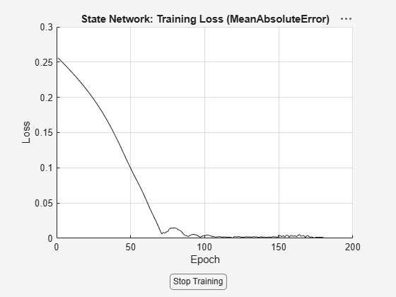
Generating estimation report...done.
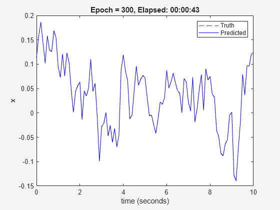
The validation plot shows that the resulting system is able to reproduce well the validation data.
Compare the Estimated System to the Original Linear System
Define a random input and initial condition.
x0 = 0.3*randn(1,1);
u0 = 0.3*randn(1,1);
Calculate the next state according to the linear system equation.
sys.a*x0 + sys.b*u0
ans =
-0.3402
Evaluate nss at the point defined by x0 and u0.
evaluate(nss,x0,u0)
ans =
-0.3405
The value of the next state calculated by evaluating nss is close to the one calculated by evaluating the linear system equation.
Display the linear system.
sys
sys =

  A =
           x1
   x1  0.9048

  B =
            u1
   x1  0.09516

  C =
       x1
   y1   1

  D =
       u1
   y1   0

Sample time: 0.1 seconds
Discrete-time state-space model.
Model Properties
Linearize nss around zero.
linearize(nss,0,0)
ans =

  A =
           x1
   x1  0.9057

  B =
            u1
   x1  0.09473

  C =
       x1
   y1   1

  D =
       u1
   y1   0

Sample time: 0.1 seconds
Discrete-time state-space model.
Model Properties
The linearized system matrices are close to the ones of the original system.
Perform an Extra Validation Check
Create input time series and a random initial state.
t = (0:Ts:10)';
u = 0.5*randn(size(t));
x0 = 0.5*randn(1,1);
Simulate both the linear and neural state-space system with the same input data, from the same initial state.
% Simulate original system from x0
ylin = lsim(sys,u,t,x0);

% Simulate neural state-space system from x0
simOpt = simOptions('InitialCondition',x0);
yn = sim(nss,array2timetable(u,RowTimes=seconds(t)),simOpt);
Note that you can also use the following code to simulate nss.
x = zeros(size(t)); x(1)=x0;
for k = 1:length(t)-1, x(k+1) = evaluate(nss,x(k),u(k)); end
Plot the outputs of both systems, also display the norm of the difference in the plot title.
stairs(t,[ylin yn.Variables]);
xlabel("Time"); ylabel("State");
legend("Original","Estimated");
title(['Approximation error =  ' num2str(norm(ylin-yn.Variables)) ])
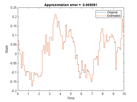
The two outputs are similar, confirming that the identified system is a good approximation of the original one.
This example shows how to estimate a nonlinear neural-state space model with no inputs and a two-dimensional continuous state equal to the output. First, you collect identification and validation data by simulating a Van der Pol system, then use the collected data to estimate and validate a neural state-space system, and finally compare the estimated system to the original system used to produce the data.
Define Model for Data Collection
Define a time-invariant continuous-time autonomous model that can be easily simulated to collect data. For this example, use an unforced Van der Pol oscillator (VDP) system, which is an oscillator with nonlinear damping that exhibits a limit cycle.
Specify the state equation using an anonymous function, using a damping coefficient of 1.
dx = @(x) [x(2); 1*(1-x(1)^2)*x(2)-x(1)];
Generate Data Set for Identification
Fix the random generator seed for reproducibility.
rng("default");Run 1000 simulations each starting at a different initial state and lasting 2 seconds. Each experiment must use identical time points.
N = 1000;
t = (0:0.1:2)';
Y = cell(1,N);

for i=1:N

    % Create random initial state within [-2,2]
    x0 = 4*rand(2,1)-2;

    % Obtain state measurements over t (solve using ode45)
    [~, x] = ode45(@(t,x) dx(x),t,x0);

    % Each experiment in the data set is a timetable
    Y{i} = array2timetable(x,RowTimes=seconds(t));

end
Generate Data Set for Validation
Run one simulation to collect data that will be used to visually inspect training result during the identification progress. The validation data set can have different time points. For this example, use the trained model to predict VDP behavior for 10 seconds.
% Create random initial state within [-2,2]
t = (0:0.1:10)';
x0 = 4*rand(2,1)-2;

% Obtain state measurements over t (solve using ode45)
[~, x] = ode45(@(t,x) dx(x),t,x0);

% Append the validation experiment (also a timetable) as the last entry in the data set
Y{end+1} = array2timetable(x,RowTimes=seconds(t));
Create a Neural State-Space Object
Create time-invariant continuous-time neural state-space object with a two-element state vector identical to the output, and no input.
nss = idNeuralStateSpace(2);
Configure State Network
Define the neural network that approximates the state function as having two hidden layers with 12 neurons each, and hyperbolic tangent activation function.
Use createMLPNetwork to create the network and dot notation to assign it to the StateNetwork property of nss.
nss.StateNetwork = createMLPNetwork(nss,'state', ...
    LayerSizes=[12 12], ...
    Activations="tanh", ...
    WeightsInitializer="glorot", ...
    BiasInitializer="zeros");
Display the number of network parameters.
summary(nss.StateNetwork)
   Initialized: true

   Number of learnables: 218

   Inputs:
      1   'x'   2 features
Specify the training options for the state network. Use the Adam algorithm and specify the maximum number of epochs as 280 (an epoch is the full pass of the training algorithm over the entire training set).
opt = nssTrainingOptions('adam');
opt.MaxEpochs = 280;
Also specify the learning rate.
opt.LearnRate = 0.015;
Estimate the Neural State-Space System
Use nlssest to train the state network of nss, using the identification data set and the predefined set of optimization options.
nss = nlssest([],Y,nss,opt,'UseLastExperimentForValidation',true);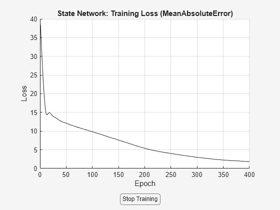
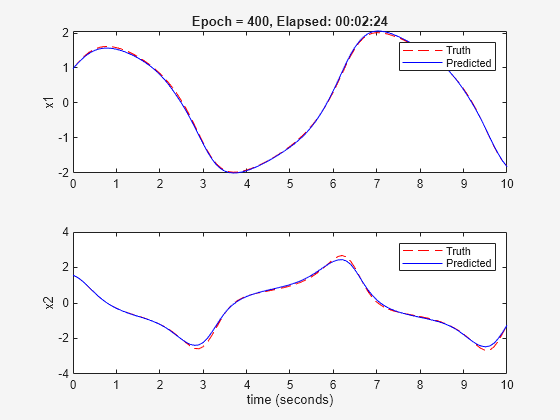
Generating estimation report...done.
The validation plot shows that the resulting system is able to reproduce well the validation data.
Compare the Estimated System to the Original Linear System
Define a random initial condition.
x0 = 0.3*randn(2,1);
Calculate the state derivative according to the original system equation.
dx(x0)
ans = 2×1

    0.0113
   -0.0325
Evaluate nss at x0.
evaluate(nss,x0)
ans = 2×1

   -0.0381
    0.0050
The value of the state derivative calculated by evaluating nss is close to the one calculated by evaluating the original system equation.
You can linearize nss around an operating point, and apply linear control analysis and synthesis methods on the resulting linear time-invariant state-space system.
sys = linearize(nss,x0)
sys =

  A =
           x1      x2
   x1  0.0336   1.028
   x2  -0.989   1.002

  B =
     Empty matrix: 2-by-0

  C =
       x1  x2
   y1   1   0
   y2   0   1

  D =
     Empty matrix: 2-by-0

Continuous-time state-space model.
Model Properties
Simulate the Neural State-Space System
Create a time sequence and a random initial state.
t = (0:0.1:10)';
x0 = 0.3*randn(2,1);
Simulate both the original and neural state-space system with the same input data, from the same initial state.
% Simulate original system from x0
[~, x] = ode45(@(t,x) dx(x),t,x0);

% Simulate neural state-space system from x0
simOpt = simOptions('InitialCondition',x0,'OutputTimes',t);
xn = sim(nss,zeros(length(t),0),simOpt);
Plot the outputs of both systems, also display the norm of the difference in the plot title.
figure;
subplot(2,1,1)
plot(t,x(:,1),t,xn(:,1));
ylabel("States(1)");
legend("Original","Estimated");
title(['Approximation error =  ' num2str(norm(x-xn)) ])
subplot(2,1,2)
plot(t,x(:,2),t,xn(:,2));
xlabel("Time"); ylabel("States(2)");
legend("Original","Estimated");
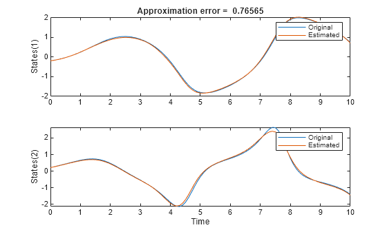
The two outputs are similar, confirming that the identified system is a good approximation of the original one.
Input Arguments
Name-Value Arguments
Output Arguments
Version History
Introduced in R2022bSee Also
Objects
idNeuralStateSpace|nssTrainingADAM|nssTrainingSGDM|nssTrainingRMSProp|nssTrainingLBFGS|idss|idnlgrey
Functions
nlssinit|createMLPNetwork|setNetwork|nssTrainingOptions|generateMATLABFunction|idNeuralStateSpace/evaluate|idNeuralStateSpace/linearize|sim
Blocks
Live Editor Tasks
Topics
- What Are Neural State-Space Models?
- Training Neural State-Space Models
- Estimate Neural State-Space System
- Estimate Nonlinear Autonomous Neural State-Space System
- Estimate Nonlinear Autonomous Neural State-Space System Using Mini-Batch Learning
- Neural State-Space Model of Simple Pendulum System
- Reduced Order Modeling of a Nonlinear Dynamical System Using Neural State-Space Model with Autoencoder
- Augment Known Linear Model with Flexible Nonlinear Functions