rf.Amplifier
Model nonlinear amplifiers using cubic polynomial, AM/AM-AM/PM, modified Rapp, or Saleh representations
Since R2024b
Description
Use the rf.Amplifier
System object™ to create an idealized amplifier for command line simulation. The
rf.Amplifier
System object is a complex baseband model of an idealized amplifier with thermal noise. This
System object provides four nonlinearity models and three options to specify noise
representation. The four nonlinearity models are cubic polynomial, AM/AM-AM/PM, modified Rapp,
and Saleh.
To create a complex baseband model of amplifier with noise and nonlinearities:
Create the
rf.Amplifierobject and set its properties.Call the object with arguments, as if it were a function.
To learn more about how System objects work, see What Are System Objects?
Creation
Description
creates an idealized
amplifier that allows you to process complex baseband signals with noise and
nonlinearities.rfamp = rf.Amplifier
sets properties of the rfamp = rf.Amplifier(Name=Value)rf.Amplifier object using one or more name-value
arguments. For example, rfamp = rf.Amplifier(Model='ampm') creates an
idealized amplifier element designed using AM/AM—AM/PM data. Properties you do not specify
retain their default values.
Properties
Unless otherwise indicated, properties are nontunable, which means you cannot change their
values after calling the object. Objects lock when you call them, and the
release function unlocks them.
If a property is tunable, you can change its value at any time.
For more information on changing property values, see System Design in MATLAB Using System Objects.
Model
Specify the amplifier nonlinearity model as one of the following:
poly— Use this model to concurrently model multiple nonlinear parameters within the idealized amplifier architecture. (since R2026a)cubic— Use this model to determine the linear coefficient of a third‑order polynomial and either IP3, P1dB, or Psat to determine the third‑order coefficient. The cubic polynomial model uses linear power gain to determine the values.ampm— Use this model to apply an AM/AM–AM/PM lookup table for computing the amplifier power characteristics.modified-rapp— Use this model to apply a normalized transfer function to compute the amplifier power characteristics.saleh— Use this model to apply a normalized transfer function based on the Saleh formulation to compute the amplifier power characteristics.
For more information, see Nonlinearity Models in Idealized Amplifier Block (RF Blockset).
Polynomial
Linear power gain for a cubic amplifier model, specified as a real number in dB.
To enable this property, set Model to
cubic.
Dependencies
To enable this property, either set Model to
'poly' or 'cubic'.
Third order nonlinearity type for the cubic amplifier model, specified as
IIP3, OIP3, IP1dB,
OP1dB, IPsat, or OPsat.
Dependencies
To enable this property, set Model to
cubic.
Input third-order intercept point, specified as a real positive number in dBm.
Dependencies
To enable this property, set Model to
'cubic' and Nonlinearity to
'IIP3'.
Output third-order intercept point, specified as a real positive number in dBm.
Dependencies
To enable this property, set either one of these:
Modelto'cubic'andNonlinearityto'OIP3'Modelto'poly'
.
Input 1 dB compression point, specified as a real positive number in dBm.
Dependencies
To enable this property, set Model to
'cubic' and Nonlinearity to
'IP1dB'.
Output 1 dB compression point, specified as a real positive number in dBm.
Dependencies
To enable this property, set either one of these:
Modelto'cubic'andNonlinearityto'OP1dB'Modelto'poly'
.
Input saturation point, specified as a real positive number in dBm.
Dependencies
To enable this property, set either one of these:
Modelto'cubic'andNonlinearityto'IPsat'Modelto'poly'
.
Output saturation point, specified as a positive real number in dBm.
Dependencies
To enable this property, set either one of these:
Modelto'cubic'andNonlinearityto'OPSat'Modelto'poly'
.
AM/AM - AM/PM
AM/AM - AM/PM lookup table entries, specified as a real M-by-3 matrix. This matrix expresses the output power in dBm in the second column and the phase change in degrees in the third column. The values in the second and third columns are relative to the absolute value of the input signal power in dBm in the first column. The values in the first column must increase monotonically.
Dependencies
To enable this property, set Model to
ampm.
Modified Rapp
Magnitude gain for the modified Rapp amplifier model AM/AM calculations, specified as a real positive number in dB.
Dependencies
To enable this property, set Model to
modified-rapp.
Voltage output saturation level for the modified Rapp amplifier model, specified as a real positive number in dBm.
Dependencies
To enable this property, set Model to
modified-rapp.
Magnitude smoothness factor for the modified Rapp amplifier model in AM/AM calculations, specified as a positive real number.
Dependencies
To enable this property, set Model to
modified-rapp.
Phase gain for the modified Rapp amplifier model in AM/PM calculations, specified as a real scalar in radians.
Dependencies
To enable this property, set Model to
modified-rapp.
Phase saturation for the modified Rapp amplifier model in AM/PM calculations, specified as a positive real number.
Dependencies
To enable this property, set Model to
modified-rapp.
Phase smoothness factor for the modified Rapp amplifier model in AM/PM calculations, specified as a positive real scalar or two-tuple vector.
Dependencies
To enable this property, set Model to
modified-rapp.
Saleh
Input signal level scaling factor for the Saleh amplifier model, specified as a real number in dB.
Dependencies
To enable this property, set Model to
saleh.
AM/AM 2-tuple [alpha beta] conversion parameters for the Saleh amplifier model, specified as a two-element row vector of real scalars.
Dependencies
To enable this property, set Model to
saleh.
AM/PM 2-tuple [alpha beta] conversion parameters for the Saleh amplifier model, specified as a two-element row vector of real scalars.
Dependencies
To enable this property, set Model to
saleh.
Output signal level scaling factor for the Saleh amplifier model, specified as real number in dB.
Dependencies
To enable this property, set Model to
saleh.
Noise Properties
Options to add system noise to the input signal, specified as a logical 1
(true) or 0 (false).
Noise representation method, specified as noise-temperature,
NF, or noise-factor.
For more information, see Thermal Noise Simulations in Idealized Amplifier Block (RF Blockset).
Dependencies
To enable this property, set IncludeNoise to
1 or true.
Noise temperature to model noise in the amplifier, specified as a nonnegative real number in degrees (K).
Dependencies
To enable this property, set IncludeNoiseto 1 or
true and set NoiseType to
noise-temperature.
Noise figure to model noise in the amplifier, specified as a nonnegative real number in dB.
Dependencies
To enable this property, set IncludeNoiseto 1 or
true and set NoiseType to
NF.
Noise factor to model noise in the amplifier, specified as a positive integer scalar greater than or equal to 1.
Dependencies
To enable this property, set IncludeNoiseto 1 or
true and set NoiseType to
noise-factor.
Source of initial seed used to prepare the Gaussian random number noise generator, specified as one of the following:
auto— Automatically generate seeds for each amplifier instance using a random number generator. The reset method of the instance has no effect.user— Use the value specified in theSeedproperty to initialize the random number generator. The reset method resets the random number generator and uses the value specified in theSeedproperty to initialize it.
Dependencies
To enable this property, set IncludeNoise to
1 or true.
Seed to initialize the random number generator, specified as either:
Scalar — Specify the seed value as a scalar to enable all the RF channel have the same Seed value.
Row vector — Specify the seed value as a row vector to enable different seed for each channel (since R2026a)
Dependencies
To enable this property, set IncludeNoise to
1 or true and set
SeedSource to user.
Sample rate, specified as a nonnegative integer of data type double in samples per second.
Dependencies
To enable this property, set IncludeNoise to
1 or true.
Usage
Syntax
Description
Input Arguments
Input baseband signal, specified as a scalar, column, or a matrix of real or complex values.
Data Types: double | single
Output
Output baseband signal, returned as a scalar, column, or a matrix of real or
complex values. The output port mimics the properties of the input port. For example,
if the input baseband signal is specified as a real scalar with data type
double, then the output baseband signal is also specified as a
real signal with data type double.
Data Types: double | single
Object Functions
To use an object function, specify the
System object as the first input argument. For
example, to release system resources of a System object named obj, use
this syntax:
release(obj)
Examples
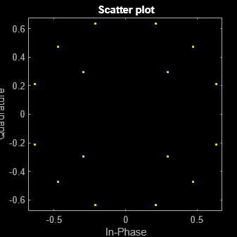
Create an rf.Amplifier System object.
rfAmp = rf.Amplifier('IPsat',30);Generate modulated symbols.
in = qammod(randi([0 15],1000,1),16,'UnitAveragePower',true);Apply the nonlinearity model to the signal and plot the results.
out = rfAmp(in); scatterplot(out)

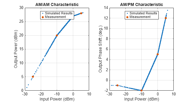
Define modulation order, samples per symbol, and input power.
M = 16; sps = 4; pindBm = 0;
Create an rf.Amplifier System object defined using an AM/AM-AM/PM nonlinearity model.
rfamp = rf.Amplifier('Model','ampm');
Apply pulse shaping by interpolating an input signal using a raised cosine finite impulse response (FIR) filter.
txfilter = comm.RaisedCosineTransmitFilter('RolloffFactor',0.3,... 'FilterSpanInSymbols',6,'OutputSamplesPerSymbol',sps,'Gain',sqrt(sps));
Define input signal.
pin = 10.^((pindBm-30)/10); % Unit: W
data = randi([0 M-1],1000,1);Define the modulated, filtered, and amplified signal.
modSig = qammod(data,M,'UnitAveragePower',true)*sqrt(pin);
filtSig = txfilter(modSig);
ampSig = rfamp(filtSig);Calculate the amplified output signal.
poutdBm = (20*log10(abs(ampSig)))+30; simulated_pindBm = (20*log10(abs(filtSig)))+30; phase = angle(ampSig .* conj(filtSig)) * 180/pi;
Plot the AM/AM-AM/PM characteristic of the amplifier by plotting the input vs. output power in a dBm plot.
figure set(gcf,'units','normalized','position',[.25 1/3 .5 1/3]) subplot (1,2,1) pow_idx = simulated_pindBm>-30; plot(simulated_pindBm(pow_idx), poutdBm(pow_idx),'.') hold on plot(rfamp.Table(:,1),rfamp.Table(:,2),'.','Markersize',15) xlabel('Input Power (dBm)') ylabel('Output Power (dBm)') grid on title('AM/AM Characteristic') Legend = {'Simulated Results','Measurement'}; legend (Legend, 'Location' , 'north')
Plot the input power (dBm) vs. output phase shift (deg).
subplot(1,2,2) plot(simulated_pindBm(pow_idx),phase(pow_idx),'.') hold on plot(rfamp.Table(:,1),rfamp.Table(:,3),'.','Markersize',15) legend(Legend,'Location','north') xlabel('Input Power (dBm)') ylabel('Output Phase Shift (deg.)') grid on title('AM/PM Characteristic')

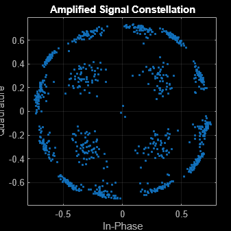
Plot the amplified signal in a constellation plot.
scatterplot(ampSig,sps,0,'.') grid on title('Amplified Signal Constellation')

This example shows how to input a two-tone signal to an idealized system. To design this RF system:
First, generate a two-tone source.
Second, connect this two-tone source to an idealized RF PA.
Finally, observe the output response of this system.
Introduction
The RF system designed in this example uses the Idealized Baseband System object™ to analyze a cascade of mathematical models of RF components within the MATLAB® environment. During analysis, these System objects uses complex-baseband representation of the RF elements to compute time-domain waveforms. These complex modulated signals represent the transmitted information, assumed to be centered around an implicit carrier frequency. The models from the Idealized Baseband library do not model out-of-band behavior or spurious harmonics generated by nonlinear effects or interfering signals. Additionally, models from the Idealized Baseband library do not model impedance mismatches and assume that all blocks are perfectly matched. As a result, RF models built with the Idealized Baseband library simulate rapidly.
Create Two-Tone Source Generator
This figure shows the architecture of a two-tone source generator. This generator consists of a sine wave generator that produces two sinusoidal signals. These signals are multiplied by a -40 dB gain and then processed by a summer.

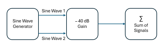
Define sample rate and samples per frame of the sine wave signals.
sampleRate = 1/2e-8; samplesPerFrame = 512;
Define a gain of - 40 dB.
m40dB = 10^(-40/20);
Create two sinusoid signals at 1.8 GHz and 2.6 GHz.
SineObj1 = dsp.SineWave('Frequency',1.8e6,'SampleRate',sampleRate, ... SamplesPerFrame=samplesPerFrame,ComplexOutput=true); SineObj2 = dsp.SineWave('Frequency',2.6e6,'SampleRate',sampleRate, ... SamplesPerFrame=samplesPerFrame,ComplexOutput=true);
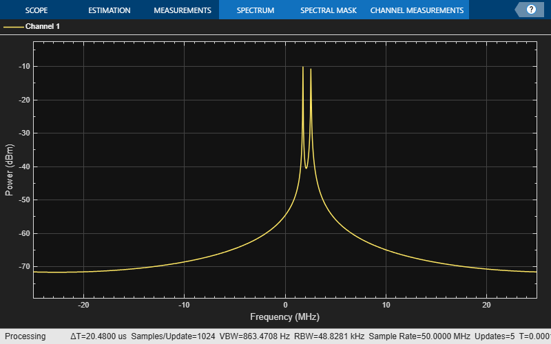
Display the spectral analysis of a two tone signal source, where each tone is -10 dBm.
SpectAnal = spectrumAnalyzer('SampleRate',sampleRate,'ShowLegend',true); for Iter = 1:10 sineWave1 = SineObj1(); sineWave2 = SineObj2(); sigIn = m40dB*(sineWave1 + sineWave2); SpectAnal(sigIn); end

Simulate Idealized System
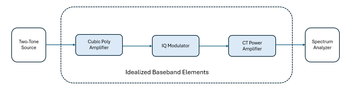
This figure shows how to create a system to IQ modulate the two-tone signal and amplify using an RF PA. The system architecture involves connecting a cubic polynomial amplifier to an IQ modulator. The output from the IQ modulator is then connected to a cross-term (CT) memory power amplifier. A two-tone signal is supplied as input to the system, and the output is connected to a spectrum analyzer for visualizing the power amplifier characteristics.

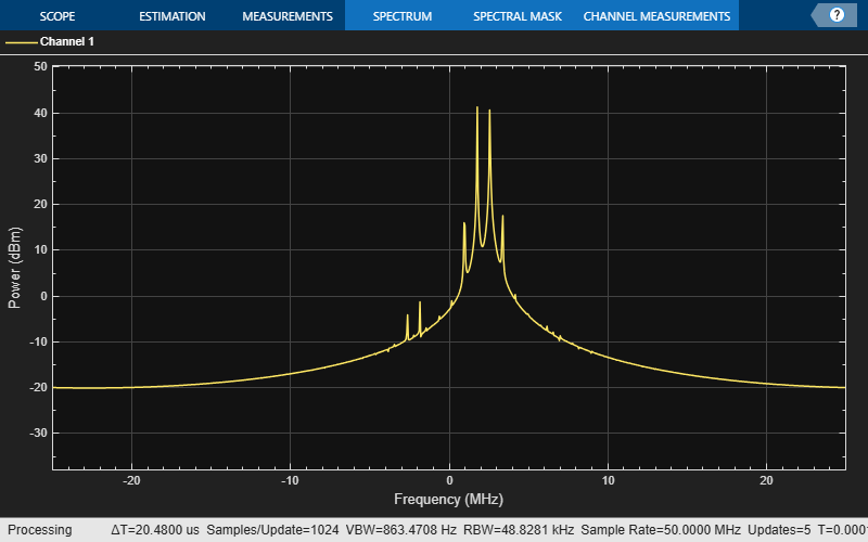
Load the pre-computed PA coefficient matrix.
load('PAcoefficients_rf.mat','fitCoefMat')
Create an idealized baseband cubic polynomial amplifier and IQ modulator with nonlinearity and noise.
preAmpIQ = rf.Amplifier('Model','cubic','Gain',8,'Nonlinearity','IIP3','IIP3',45, ... 'IncludeNoise',true,NF=1.5); mixerModIQ = rf.Mixer('Model','iqmod','Gain',0,'LO',1e8, ... 'PhaseImbalance',.5,'Nonlinearity','IIP3',IIP3=50, ... IncludeNoise=true,NoiseType='NF',NF=6);
Create an idealized baseband cross-term memory PA.
powerAmp = rf.PAmemory('Model','Cross-term memory', ... 'CoefficientMatrix','fitCoefMat');
Connect the RF chain and provide the two-tone signal as input.
SpectAnal = spectrumAnalyzer('SampleRate',sampleRate,'ShowLegend',true); for Iter = 1:10 sineWave1 = SineObj1(); sineWave2 = SineObj2(); sineIn = m40dB*(sineWave1 + sineWave2); ampIQ = preAmpIQ(sineIn); modIQ = mixerModIQ(ampIQ); paOut = powerAmp(modIQ*sqrt(50))/sqrt(50); SpectAnal(paOut); end

References
[1] Razavi, Behzad. “Basic Concepts “ in RF Microelectronics, 2nd edition, Prentice Hall, 2012.
[2] Rapp, C., “Effects of HPA-Nonlinearity on a 4-DPSK/OFDM-Signal for a Digital Sound Broadcasting System.” Proceedings of the Second European Conference on Satellite Communications, Liege, Belgium, Oct. 22-24, 1991, pp. 179-184.
[3] Saleh, A.A.M., “Frequency-independent and frequency-dependent nonlinear models of TWT amplifiers.” IEEE Trans. Communications, vol. COM-29, pp.1715-1720, November 1981.
[4] IEEE 802.11-09/0296r16. “TGad Evaluation Methodology.“ Institute of Electrical and Electronics Engineers.https://www.ieee.org/
[5] Kundert, Ken.“ Accurate and Rapid Measurement of IP2 and IP3,“ The Designer Guide Community, May 22, 2002.
Version History
Introduced in R2024bConfigure the idealized rf.Amplifier object
with the poly model type to concurrently model multiple nonlinear
parameters within the idealized amplifier architecture.
Starting in R2026a, the default value of the Model property in
the rf.Amplifier system object has changed from
‘cubic’ to ‘poly’.
When creating an rf.Amplifier object in R2026a,
‘poly’ is now the default setting for the Model property.
The rf.amplifier object now supports matrix inputs to enable the
simulation of multiple independent RF channels concurrently within the Idealized Baseband
simulation environment.
MATLAB Command
You clicked a link that corresponds to this MATLAB command:
Run the command by entering it in the MATLAB Command Window. Web browsers do not support MATLAB commands.
Select a Web Site
Choose a web site to get translated content where available and see local events and offers. Based on your location, we recommend that you select: .
You can also select a web site from the following list
How to Get Best Site Performance
Select the China site (in Chinese or English) for best site performance. Other MathWorks country sites are not optimized for visits from your location.
Americas
- América Latina (Español)
- Canada (English)
- United States (English)
Europe
- Belgium (English)
- Denmark (English)
- Deutschland (Deutsch)
- España (Español)
- Finland (English)
- France (Français)
- Ireland (English)
- Italia (Italiano)
- Luxembourg (English)
- Netherlands (English)
- Norway (English)
- Österreich (Deutsch)
- Portugal (English)
- Sweden (English)
- Switzerland
- United Kingdom (English)