Nichols Plot
Nichols plot of linear system approximated from nonlinear Simulink model
Library
Simulink® Control Design™
Description
This block is the same as the Check Nichols Characteristics block except for different default parameter settings in the Bounds tab.
Compute a linear system from a nonlinear Simulink model and plot the linear system on a Nichols plot.
During simulation, the software linearizes the portion of the model between specified linearization inputs and outputs, and plots the open-loop gain and phase of the linear system.
The Simulink model can be continuous- or discrete-time or multirate and can have time delays. Because you can specify only one linearization input/output pair in this block, the linear system is Single-Input Single-Output (SISO).
You can specify multiple open- and closed-loop gain and phase bounds and view them on the Nichols plot. You can also check that the bounds are satisfied during simulation:
If all bounds are satisfied, the block does nothing.
If a bound is not satisfied, the block asserts and a warning message appears in the MATLAB® Command Window. You can also specify that the block:
Evaluate a MATLAB expression.
Stop the simulation and bring that block into focus.
During simulation, the block can also output a logical assertion signal.
If all bounds are satisfied, the signal is true (
1).If any bound is not satisfied, the signal is false (
0).
You can add multiple Nichols Plot blocks to compute and plot the gains and phases of various portions of the model.
You can save the linear system as a variable in the MATLAB workspace.
The block does not support code generation and can be used only
in Normal simulation mode.
Parameters
The following table summarizes the Nichols Plot block parameters, accessible via the block parameter dialog box.
| Task | Parameters | |
|---|---|---|
| Configure linearization. | Specify inputs and outputs (I/Os). |
In Linearizations tab: |
| Specify settings. |
In Linearizations tab: | |
| Specify algorithm options. |
In Algorithm Options of Linearizations tab: | |
| Specify labels for linear system I/Os and state names. |
In Labels of Linearizations tab: | |
| Plot the linear system. | Show Plot | |
| Specify the feedback sign for closed-loop gain and phase margins. | Feedback sign in Bounds tab. | |
| (Optional) Specify bounds on gains and phases of the linear system for assertion. |
In Bounds tab: | |
| Specify assertion options (only when you specify bounds on the linear system). |
In Assertion tab: | |
| Save linear system to MATLAB workspace. | Save data to workspace in Logging tab. | |
| Display plot window instead of block parameters dialog box on double-clicking the block. | Show plot on block open. | |
Linearization inputs/outputs
Linearization inputs and outputs that define the portion of a nonlinear Simulink model to linearize.
If you have defined the linearization input and output in the Simulink model,
the block automatically detects these points and displays them in
the Linearization inputs/outputs area. Click ![]() at any time to update
the Linearization inputs/outputs table with I/Os
from the model. To add other analysis points:
at any time to update
the Linearization inputs/outputs table with I/Os
from the model. To add other analysis points:
Click
 .
. The dialog box expands to display a Click a signal in the model to select it area and a new
 button.
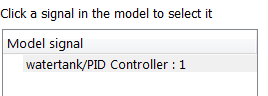
Select one or more signals in the Simulink Editor.
The selected signals appear under Model signal in the Click a signal in the model to select it area.
(Optional) For buses, expand the bus signal to select individual elements.
Tip
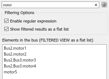
For large buses or other large lists of signals, you can enter search text for filtering element names in the Filter by name edit box. The name match is case-sensitive. Additionally, you can enter a MATLAB regular expression.
To modify the filtering options, click
 . To hide the filtering
options, click
. To hide the filtering
options, click  .
.Click
to add the selected signals to the
Linearization inputs/outputs table.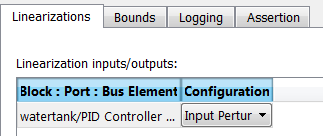
To remove a signal from the Linearization inputs/outputs table, select the signal and click
 .
.Tip
To find the location in the Simulink model corresponding to a signal in the Linearization inputs/outputs table, select the signal in the table and click
 .
.
The table displays the following information about the selected signal:
| Block : Port : Bus Element | Name of the block associated with the input/output. The number adjacent to the block name is the port number where the selected bus signal is located. The last entry is the selected bus element name. |
| Configuration |
Type of linearization point:
|
Note
If you simulate the model without specifying an input or output, the software does not compute a linear system. Instead, you see a warning message at the MATLAB prompt.
No default
Click a signal in the model to select it
Enables signal selection in the Simulink model. Appears
only when you click ![]() .
.
When this option appears, you also see the following changes:
A new
button.Use to add a selected signal as a linearization input or output in the Linearization inputs/outputs table. For more information, see Linearization inputs/outputs.
- changes to
 .
.Use
to collapse the Click
a signal in the model to select it area.
No default
Enable regular expression
Enable the use of MATLAB regular expressions for filtering
signal names. For example, entering t$ in the Filter
by name edit box displays all signals whose names end with
a lowercase t (and their immediate parents). For
details, see Regular Expressions.
Default: On
 On
On Allow use of MATLAB regular expressions for filtering signal names.
 Off
OffDisable use of MATLAB regular expressions for filtering signal names. Filtering treats the text you enter in the Filter by name edit box as a literal character vector.
Selecting the Options button on the right-hand
side of the Filter by name edit box
(![]() ) enables this parameter.
) enables this parameter.
Show filtered results as a flat list
Uses a flat list format to display the list of filtered signals, based on the search text in the Filter by name edit box. The flat list format uses dot notation to reflect the hierarchy of bus signals. The following is an example of a flat list format for a filtered set of nested bus signals.
Default: Off
- On
Display the filtered list of signals using a flat list format, indicating bus hierarchies with dot notation instead of using a tree format.
- Off
Display filtered bus hierarchies using a tree format.
Selecting the Options button on the right-hand
side of the Filter by name edit box
(![]() ) enables this parameter.
) enables this parameter.
Linearize on
When to compute the linear system during simulation.
Default: Simulation
snapshots
Simulation snapshotsSpecific simulation time, specified in Snapshot times.
Use when you:
Know one or more times when the model is at a steady-state operating point
Want to compute the linear systems at specific times
External triggerTrigger-based simulation event. Specify the trigger type in Trigger type.
Use when a signal generated during simulation indicates steady-state operating point.
Selecting this option adds a trigger port to the block. Use this port to connect the block to the trigger signal.
For example, for an aircraft model, you might want to compute the linear system whenever the fuel mass is a fraction of the maximum fuel mass. In this case, model this condition as an external trigger.
Setting this parameter to
Simulation
snapshots
enables Snapshot times.Setting this parameter to
External triggerenables Trigger type.
Parameter: LinearizeAt |
| Type: character vector |
Value: 'SnapshotTimes' | 'ExternalTrigger' |
Default: 'SnapshotTimes' |
Snapshot times
One or more simulation times. The linear system is computed at these times.
Default: 0
For a different simulation time, enter the time. Use when you:
Want to plot the linear system at a specific time
Know the approximate time when the model reaches steady-state operating point
For multiple simulation times, enter a vector. Use when you want to compute and plot linear systems at multiple times.
Snapshot times must be less than or equal to the simulation time specified in the Simulink model.
Selecting Simulation snapshots in Linearize on enables
this parameter.
Parameter: SnapshotTimes |
| Type: character vector |
Value: 0 |
positive real number | vector of positive real numbers |
Default: 0 |
Trigger type
Trigger type of an external trigger for computing linear system.
Default: Rising
edge
Rising
edge
Rising edge of the external trigger signal.
Falling edgeFalling edge of the external trigger signal.
Selecting External trigger in Linearize on enables
this parameter.
Parameter: TriggerType |
| Type: character vector |
Value: 'rising' | 'falling' |
Default: 'rising' |
Enable zero-crossing detection
Enable zero-crossing detection to ensure that the software computes the linear system characteristics at the following simulation times:
The exact snapshot times, specified in Snapshot times.
As shown in the following figure, when zero-crossing detection is enabled, the variable-step Simulink solver simulates the model at the snapshot time
Tsnap.Tsnapmay lie between the simulation time stepsTn-1andTnwhich are automatically chosen by the solver.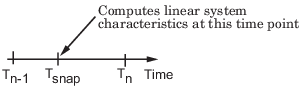
The exact times when an external trigger is detected, specified in Trigger type.
As shown in the following figure, when zero-crossing detection is enabled, the variable-step Simulink solver simulates the model at the time,
Ttrig, when the trigger signal is detected.Ttrigmay lie between the simulation time stepsTn-1andTnwhich are automatically chosen by the solver.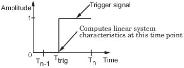
For more information on zero-crossing detection, see Zero-Crossing Detection in the Simulink User Guide.
Default: On
- On
Compute linear system characteristics at the exact snapshot time or exact time when a trigger signal is detected.
This setting is ignored if the Simulink solver is fixed step.
- Off
Compute linear system characteristics at the simulation time steps that the variable-step solver chooses. The software may not compute the linear system at the exact snapshot time or exact time when a trigger signal is detected.
Parameter: ZeroCross |
| Type: character vector |
Value: 'on' | 'off' |
Default: 'on' |
Use exact delays
How to represent time delays in your linear model.
Use this option if you have blocks in your model that have time delays.
Default: Off
- On
Return a linear model with exact delay representations.
- Off
Return a linear model with Padé approximations of delays, as specified in your Transport Delay and Variable Transport Delay blocks.
Parameter: UseExactDelayModel |
| Type: character vector |
Value: 'on' | 'off' |
Default: 'off' |
Linear system sample time
Sample time of the linear system computed during simulation.
Use this parameter to:
Compute a discrete-time system with a specific sample time from a continuous-time system
Resample a discrete-time system with a different sample time
Compute a continuous-time system from a discrete-time system
When computing discrete-time systems from continuous-time systems and vice-versa, the software uses the conversion method specified in Sample time rate conversion method.
Default: auto
auto. Computes the sample time as:0, for continuous-time models.
For models that have blocks with different sample times (multirate models), least common multiple of the sample times. For example, if you have a mix of continuous-time and discrete-time blocks with sample times of 0, 0.2 and 0.3, the sample time of the linear model is 0.6.
- Positive finite value. Use to compute:
A discrete-time linear system from a continuous-time system.
A discrete-time linear system from another discrete-time system with a different sample time.
0Use to compute a continuous-time linear system from a discrete-time model.
Parameter: SampleTime |
| Type: character vector |
Value:
'auto' | Positive finite value | '0' |
Default:
'auto' |
Sample time rate conversion method
Method for converting the sample time of single-rate or multirate models.
This parameter is used only when the value of Linear
system sample time is not auto.
Default: Zero-Order
Hold
Zero-Order HoldZero-order hold, where the control inputs are assumed piecewise constant over the sampling time
Ts. For more information, see Zero-Order Hold.This method usually performs better in the time domain.
Tustin (bilinear)Bilinear (Tustin) approximation without frequency prewarping. The software rounds off fractional time delays to the nearest multiple of the sampling time. For more information, see Tustin Approximation.
This method usually performs better in the frequency domain.
Tustin with PrewarpingBilinear (Tustin) approximation with frequency prewarping. Also specify the prewarp frequency in Prewarp frequency (rad/s). For more information, see Tustin Approximation.
This method usually performs better in the frequency domain. Use this method to ensure matching at frequency region of interest.
Upsampling when possible, Zero-Order
Hold otherwise
Upsample a discrete-time system when possible and use
Zero-Order Holdotherwise.You can upsample only when you convert a discrete-time system to a new faster sample time that is an integer multiple of the sample time of the original system.
Upsampling when possible, Tustin
otherwise
Upsample a discrete-time system when possible and use
Tustin (bilinear)otherwise.You can upsample only when you convert a discrete-time system to a new faster sample time that is an integer multiple of the sample time of the original system.
Upsampling when possible, Tustin
with Prewarping otherwise
Upsample a discrete-time system when possible and use
Tustin
with Prewarping
otherwise. Also, specify the prewarp frequency in Prewarp frequency (rad/s).You can upsample only when you convert a discrete-time system to a new faster sample time that is an integer multiple of the sample time of the original system.
Selecting either:
Tustin with PrewarpingUpsampling when possible, Tustin with Prewarping otherwise
enables Prewarp frequency (rad/s).
Parameter: RateConversionMethod |
| Type: character vector |
Value: 'zoh' | 'tustin' | 'prewarp'| 'upsampling_zoh'| 'upsampling_tustin'| 'upsampling_prewarp' |
Default: 'zoh' |
Prewarp frequency (rad/s)
Prewarp frequency for Tustin method, specified in radians/second.
Default: 10
Positive scalar value, smaller than the Nyquist frequency before
and after resampling. A value of 0 corresponds
to the standard Tustin method without frequency prewarping.
Selecting either
Tustin with PrewarpingUpsampling when possible, Tustin with Prewarping otherwise
in Sample time rate conversion method enables this parameter.
Parameter: PreWarpFreq |
| Type: character vector |
Value: 10 |
positive scalar value |
Default: 10 |
Use full block names
How the state, input and output names appear in the linear system computed during simulation.
The linear system is a state-space object, and system states and input/output names appear in following state-space object properties:
| Input, Output or State Name | Appears in Which State-Space Object Property |
|---|---|
| Linearization input name | InputName |
| Linearization output name | OutputName |
| State names | StateName |
Default: Off
- On
Show state and input/output names with their path through the model hierarchy. For example, in the
scdcstrmodel used in the Plot Linear System Characteristics of a Chemical Reactor example, a state in theIntegrator1block of theCSTRsubsystem appears with full path asscdcstr/CSTR/Integrator1.- Off
Show only state and input/output names. Use this option when the signal name is unique and you know where the signal is location in your Simulink model. For example, a state in the
Integrator1block of theCSTRsubsystem appears asIntegrator1.
Parameter: UseFullBlockNameLabels |
| Type: character vector |
Value: 'on' | 'off' |
Default: 'off' |
Use bus signal names
How to label signals associated with linearization inputs and outputs on buses, in the linear system computed during simulation (applies only when you select an entire bus as an I/O point).
Selecting an entire bus signal is not recommended. Instead, select individual bus elements.
You cannot use this parameter when your model has mux/bus mixtures.
Default: Off
- On
Use the signal names of the individual bus elements.
Bus signal names appear when the input and output are at the output of the following blocks:
Root-level inport block containing a bus object
Bus creator block
Subsystem block whose source traces back to one of the following blocks:
Output of a bus creator block
Root-level inport block by passing through only virtual or nonvirtual subsystem boundaries
- Off
Use the bus signal channel number.
Parameter: UseBusSignalLabels |
| Type: character vector |
Value: 'on' | 'off' |
Default: 'off' |
Include gain and phase margins in assertion
Check that the gain and phase margins are greater than the values specified in Gain margin (dB) > and Phase margin (deg) >, during simulation. The software displays a warning if the gain or phase margin is less than or equal to the specified value.
By default, negative feedback, specified in Feedback sign, is used to compute the margins.
This parameter is used for assertion only if Enable assertion in the Assertion tab is selected.
You can specify multiple gain and phase margin bounds on the linear system. The bounds also appear on the Nichols plot. If you clear Enable assertion, the bounds are not used for assertion but continue to appear on the plot.
Default:
Off for Nichols Plot block.
On for Check Nichols Characteristics block.
- On
Check that the gain and phase margins satisfy the specified values, during simulation.
- Off
Do not check that the gain and phase margins satisfy the specified values, during simulation.
Clearing this parameter disables the gain and phase margin bounds and the software stops checking that the gain and phase margins satisfy the bounds during simulation. The bounds are also greyed out on the plot.
To only view the gain and phase margin on the plot, clear Enable assertion.
Parameter: EnableMargins |
| Type: character vector |
Value: 'on' | 'off' |
Default: 'off' for Nichols
Plot block, 'on' for Check Nichols
Characteristics block |
Gain margin (dB) >
Gain margin, in decibels.
By default, negative feedback, specified in Feedback sign, is used to compute the gain margin.
Default:
[] for Nichols Plot block. |
20 for Check Nichols Characteristics block. |
Positive finite number for one bound.
Cell array of positive finite numbers for multiple bounds.
To assert that the gain margin is satisfied, select both Include gain and phase margins in assertion and Enable assertion.
You can add or modify gain margins from the plot window:
To add new gain margin, right-click the plot, and select Bounds > New Bound. Select
Gain marginin Design requirement type, and specify the margin in Gain margin.To modify the gain margin, drag the segment. Alternatively, right-click the plot, and select Bounds > Edit Bound. Specify the new gain margin in Gain margin >.
You must click Update Block before simulating the model.
Parameter: GainMargin |
| Type: character vector |
Value: [] | 20 |
positive finite value. Must be specified inside single quotes (''). |
Default: '[]' for Nichols
Plot block, '20' for Check Nichols
Characteristics block. |
Phase margin (deg) >
Phase margin, in degrees.
By default, negative feedback, specified in Feedback sign, is used to compute the phase margin.
[] for Nichols Plot block. |
30 for Check Nichols Characteristics block. |
Positive finite number for one bound.
Cell array of positive finite numbers for multiple bounds.
To assert that the phase margin is satisfied, select both Include gain and phase margins in assertion and Enable assertion.
You can add or modify phase margins from the plot window:
To add new phase margin, right-click the plot, and select Bounds > New Bound. Select
Phase marginin Design requirement type, and specify the margin in Phase margin.To modify the phase margin, drag the segment. Alternatively, right-click the bound, and select Bounds > Edit Bound. Specify the new phase margin in Phase margin >.
You must click Update Block before simulating the model.
Parameter: PhaseMargin |
| Type: character vector |
Value: [] | 30 |
positive finite value. Must be specified inside single quotes (''). |
Default: '[]' for Nichols
Plot block, '30' for Check Nichols
Characteristics block. |
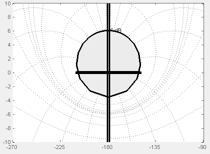
Include closed-loop peak gain in assertion
Check that the closed-loop peak gain is less than the value specified in Closed-loop peak gain (dB) <, during simulation. The software displays a warning if the closed-loop peak gain is greater than or equal to the specified value.
By default, negative feedback, specified in Feedback sign, is used to compute the closed-loop peak gain.
This parameter is used for assertion only if Enable assertion in the Assertion tab is selected.
You can specify multiple closed-loop peak gain bounds on the linear system. The bound also appear on the Nichols plot as an m-circle. If you clear Enable assertion, the bounds are not used for assertion but continue to appear on the plot.
Default: Off
- On
Check that the closed-loop peak gain satisfies the specified value, during simulation.
- Off
Do not check that the closed-loop peak gain satisfies the specified value, during simulation.
Clearing this parameter disables the closed-loop peak gain bound and the software stops checking that the peak gain satisfies the bounds during simulation. The bounds are greyed out on the plot.
To only view the closed-loop peak gain on the plot, clear Enable assertion.
Parameter: EnableCLPeakGain |
| Type: character vector |
Value: 'on' | 'off' |
Default: 'off' |
Closed-loop peak gain (dB) <
Closed-loop peak gain, in decibels.
By default, negative feedback, specified in Feedback sign, is used to compute the margins.
Default []
Positive or negative finite number for one bound.
Cell array of positive or negative finite numbers for multiple bounds.
To assert that the gain margin is satisfied, select both Include closed-loop peak gain in assertion and Enable assertion.
You can add or modify closed-loop peak gains from the plot window:
To add the closed-loop peak gain, right-click the plot, and select Bounds > New Bound. Select
Closed-Loop
peak gain
in Design requirement type, and specify the gain in Closed-Loop peak gain <.To modify the closed-loop peak gain, drag the segment. Alternatively, right-click the bound, and select Bounds > Edit Bound. Specify the new closed-loop peak gain in Closed-Loop peak gain <.
You must click Update Block before simulating the model.
Parameter: CLPeakGain |
| Type: character vector |
Value: [] |
positive or negative number | cell array of positive or negative numbers.
Must be specified inside single quotes (''). |
Default: '[]' |
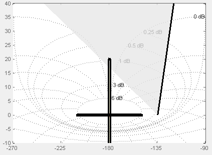
Include open-loop gain-phase bound in assertion
Check that the Nichols response satisfies open-loop gain and phase bounds, specified in Open-loop phases (deg) and Open-loop gains (dB), during simulation. The software displays a warning if the Nichols response violates the bounds.
This parameter is used for assertion only if Enable assertion in the Assertion tab is selected.
You can specify multiple gain and phase bounds on the linear systems computed during simulation. The bounds also appear on the Nichols plot. If you clear Enable assertion, the bounds are not used for assertion but continue to appear on the plot.
Default: Off
- On
Check if the Nichols response satisfies the specified open-loop gain and phase bounds, during simulation.
- Off
Do not check if the Nichols response satisfies the specified open-loop gain and phase bounds, during simulation.
Clearing this parameter disables the gain-phase bound and the software stops checking that the gain and phase satisfy the bound during simulation. The bound segments are also greyed out on the plot.
To only view the bound on the plot, clear Enable assertion.
Parameter: EnableGainPhaseBound |
| Type: character vector |
Value: 'on' | 'off' |
Default: 'off' |
Open-loop phases (deg)
Open-loop phases, in degrees.
Specify the corresponding open-loop gains in Open-loop gains (dB).
Default: []
Must be specified as start and end phases:
Positive or negative finite numbers for a single bound with one edge
Matrix of positive or negative finite numbers , for a single bound with multiple edges
Cell array of matrices with finite numbers for multiple bounds
To assert that the open-loop gains and phases are satisfied, select both Include open-loop gain-phase bound in assertion and Enable assertion.
You can add or modify open-loop phases from the plot window:
To add a new phases, right-click the plot, and select Bounds > New Bound. Select
Gain-Phase requirementin Design requirement type, and specify the phases in the Open-Loop phase column. Specify the corresponding gains in the Open-Loop gain column.To modify the phases, drag the bound segment. Alternatively, right-click the segment, and select Bounds > Edit Bounds. Specify the new phases in the Open-Loop phase column.
You must click Update Block before simulating the model.
Parameter: OLPhases |
| Type: character vector |
Value: []
| positive or negative finite numbers | matrix of positive or
negative finite numbers | cell array of matrices with finite numbers.
Must be specified inside single quotes (''). |
Default: '[]' |
Open-loop gains (dB)
Open-loop gains, in decibels.
Specify the corresponding open-loop phases in Open-loop phases (deg).
Default: []
Must be specified as start and end gains:
Positive or negative number for a single bound with one edge
Matrix of positive or negative finite numbers for a single bound with multiple edges
Cell array of matrices with finite numbers for multiple bounds
To assert that the open-loop gains are satisfied, select both Include open-loop gain-phase bound in assertion and Enable assertion.
You can add or modify open-loop gains from the plot window:
To add a new gains, right-click the plot, and select Bounds > New Bound. Select
Gain-Phase requirementin Design requirement type, and specify the gains in the Open-Loop phase column. Specify the phases in the Open-Loop phase column.To modify the gains, drag the bound segment. Alternatively, right-click the segment, and select Bounds > Edit Bounds. Specify the new gains in the Open-Loop gain column.
You must click Update Block before simulating the model.
Parameter: OLGains |
| Type: character vector |
Value: [] |
positive or negative number | matrix of positive or negative finite
numbers | cell array of matrices with finite numbers. Must be specified
inside single quotes (''). |
Default: '[]' |
Feedback sign
Feedback sign to determine the closed-loop gain and phase characteristics of the linear system, computed during simulation.
To determine the feedback sign, check if the path defined by the linearization inputs and outputs include the feedback Sum block:
If the path includes the Sum block, specify positive feedback.
If the path does not include the Sum block, specify the same feedback sign as the Sum block.
Default: negative
feedback
negative feedbackUse when the path defined by the linearization inputs/outputs does not include the Sum block and the Sum block feedback sign is
-.positive feedbackUse when:
The path defined by the linearization inputs/outputs includes the Sum block.
The path defined by the linearization inputs/outputs does not include the Sum block and the Sum block feedback sign is
+.
Parameter: FeedbackSign |
| Type: character vector |
Value: '-1' | '+1' |
Default: '-1' |
Save data to workspace
Save one or more linear systems to perform further linear analysis or control design.
The saved data is in a structure whose fields include:
time— Simulation times at which the linear systems are computed.values— State-space model representing the linear system. If the linear system is computed at multiple simulation times,valuesis an array of state-space models.operatingPoints— Operating points corresponding to each linear system invalues. This field exists only if Save operating points for each linearization is checked.
The location of the saved data structure depends upon the configuration of the Simulink model:
If the Simulink model is not configured to save simulation output as a single object, the data structure is a variable in the MATLAB workspace.
If the Simulink model is configured to save simulation output as a single object, the data structure is a field in the
Simulink.SimulationOutputobject that contains the logged simulation data.To configure your model to save simulation output in a single object, in the Simulink editor, on the Modeling tab, click Model Settings. Then, in the Configuration Parameters dialog box, select the Single simulation output parameter.
For more information about data logging in Simulink, see Save Simulation Data and the Simulink.SimulationOutput reference page.
Default: Off
- On
Save the computed linear system.
- Off
Do not save the computed linear system.
This parameter enables Variable name.
Parameter:
SaveToWorkspace |
| Type: character vector |
Value:
'on' | 'off' |
Default:
'off' |
Variable name
Name of the data structure that stores one or more linear systems computed during simulation.
The location of the saved data structure depends upon the configuration of the Simulink model:
If the Simulink model is not configured to save simulation output as a single object, the data structure is a variable in the MATLAB workspace.
If the Simulink model is configured to save simulation output as a single object, the data structure is a field in the
Simulink.SimulationOutputobject that contains the logged simulation data.
The name must be unique among the variable names used in all data logging model blocks, such as Linear Analysis Plot blocks, Model Verification blocks, Scope blocks, To Workspace blocks, and simulation return variables such as time, states, and outputs.
For more information about data logging in Simulink, see Save Simulation Data and the Simulink.SimulationOutput reference page.
Default: sys
Character vector.
Save data to workspace enables this parameter.
Parameter: SaveName |
| Type: character vector |
Value: sys |
any character vector. Must be specified inside single quotes (''). |
Default: 'sys' |
Save operating points for each linearization
When saving linear systems to the workspace for further analysis
or control design, also save the operating point corresponding to
each linearization. Using this option adds a field named operatingPoints to
the data structure that stores the saved linear systems.
Default: Off
- On
Save the operating points.
- Off
Do not save the operating points.
Save data to workspace enables this parameter.
Parameter: SaveOperatingPoint |
| Type: character vector |
Value: 'on' | 'off' |
Default: 'off' |
Enable assertion
Enable the block to check that bounds specified and included for assertion in the Bounds tab are satisfied during simulation. Assertion fails if a bound is not satisfied. A warning, reporting the assertion failure, appears at the MATLAB prompt.
If assertion fails, you can optionally specify that the block:
Execute a MATLAB expression, specified in Simulation callback when assertion fails (optional).
Stop the simulation and bring that block into focus, by selecting Stop simulation when assertion fails.
For the Linear Analysis Plots blocks, this parameter has no effect because no bounds are included by default. If you want to use the Linear Analysis Plots blocks for assertion, specify and include bounds in the Bounds tab.
Clearing this parameter disables assertion; that is, the block no longer checks that specified bounds are satisfied. The block icon also updates to indicate that assertion is disabled.
In the Simulink model, in the Configuration Parameters dialog box, the Model Verification block enabling parameter lets you enable or disable all model verification blocks in a model, regardless of the setting of this option in the block.
Default: On
- On
Check that bounds included for assertion in the Bounds tab are satisfied during simulation. A warning, reporting assertion failure, is displayed at the MATLAB prompt if bounds are violated.
- Off
Do not check that bounds included for assertion are satisfied during simulation.
This parameter enables:
Simulation callback when assertion fails (optional)
Stop simulation when assertion fails
Parameter: enabled |
| Type: character vector |
Value: 'on' | 'off' |
Default: 'on' |
Simulation callback when assertion fails (optional)
MATLAB expression to execute when assertion fails.
Because the expression is evaluated in the MATLAB workspace, define all variables used in the expression in that workspace.
No Default
A MATLAB expression.
Enable assertion enables this parameter.
Parameter: callback |
| Type: character vector |
Value: '' | MATLAB expression |
Default: '' |
Stop simulation when assertion fails
Stop the simulation when a bound specified in the Bounds tab is violated during simulation, i.e., assertion fails.
If you run the simulation from the Simulink Editor, the Simulation Diagnostics window opens to display an error message. Also, the block where the bound violation occurs is highlighted in the model.
Default: Off
- On
Stop simulation if a bound specified in the Bounds tab is violated.
- Off
Continue simulation if a bound is violated with a warning message at the MATLAB prompt.
Because selecting this option stops the simulation as soon as the assertion fails, assertion failures that might occur later during the simulation are not reported. If you want all assertion failures to be reported, do not select this option.
Enable assertion enables this parameter.
Parameter: stopWhenAssertionFail |
| Type: character vector |
Value: 'on' | 'off' |
Default: 'off' |
Output assertion signal
Output a Boolean signal that, at each time step, is:
True (
1) if assertion succeeds; that is, all bounds are satisfiedFalse (
1) if assertion fails; that is, a bound is violated.
The output signal data type is Boolean only if, in the Simulink model, in the Configuration Parameters dialog box, the Implement logic signals as Boolean data parameter is selected. Otherwise, the data type of the output signal is double.
Selecting this parameter adds an output port to the block that you can connect to any block in the model.
Default:Off
- On
Output a Boolean signal to indicate assertion status. Adds a port to the block.
- Off
Do not output a Boolean signal to indicate assertion status.
Use this parameter to design complex assertion logic. For an example, see Verify Model Using Simulink Control Design and Simulink Verification Blocks.
Parameter: export |
| Type: character vector |
Value: 'on' | 'off' |
Default: 'off' |
Show plot on block open
Open the plot window instead of the Block Parameters dialog box when you double-click the block in the Simulink model.
Use this parameter if you prefer to open and perform tasks, such as adding or modifying
bounds, in the plot window instead of the Block Parameters dialog box. If you want to access
the block parameters from the plot window, select Edit or click
![]() .
.
For more information on the plot, see Show Plot.
Default: Off
- On
Open the plot window when you double-click the block.
- Off
Open the Block Parameters dialog box when you double-click the block.
Parameter: LaunchViewOnOpen |
| Type: character vector |
Value: 'on' | 'off' |
Default: 'off' |
Show Plot
Open the plot window.
Use the plot to view:
System characteristics and signals computed during simulation
You must click this button before you simulate the model to view the system characteristics or signal.
You can display additional characteristics, such as the peak response time, by right-clicking the plot and selecting Characteristics.
Bounds
You can specify bounds in the Bounds tab of the Block Parameters dialog box or right-click the plot and select Bounds > New Bound. For more information on the types of bounds you can specify, see the individual reference pages.
You can modify bounds by dragging the bound segment or by right-clicking the plot and selecting Bounds > Edit Bound. Before you simulate the model, click Update Block to update the bound value in the block parameters.
Typical tasks that you perform in the plot window include:
Opening the Block Parameters dialog box by clicking
 or selecting Edit.
Finding the block that the plot window corresponds to by clicking
 or selecting View > Highlight Simulink Block. This action makes the model window active and highlights the
block.
or selecting View > Highlight Simulink Block. This action makes the model window active and highlights the
block.Simulating the model by clicking
 . This action also linearizes the portion of the
model between the specified linearization input and output.
. This action also linearizes the portion of the
model between the specified linearization input and output.Adding a legend on the linear system characteristic plot by clicking
 .
.
Note
To optimize the model response to meet design requirements specified in the Bounds tab, open the Response Optimizer by selecting Tools > Response Optimization in the plot window. This option is only available if you have Simulink Design Optimization™ software installed.
Response Optimization
Open the Response Optimizer to optimize the model response to meet design requirements specified in the Bounds tab.
This button is available only if you have Simulink Design Optimization software installed.
Design Optimization to Meet Step Response Requirements (GUI) (Simulink Design Optimization)
Design Optimization to Meet Time-Domain and Frequency-Domain Requirements (GUI) (Simulink Design Optimization)
See Also
Tutorials
Version History
Introduced in R2010b