Main Content

fitensemble

Fit ensemble of learners for classification and regression

Description

fitensemble can boost or bag decision tree learners or discriminant analysis classifiers. The function can also train random subspace ensembles of KNN or discriminant analysis classifiers.

For simpler interfaces that fit classification and regression ensembles, instead use fitcensemble and fitrensemble, respectively. Also, fitcensemble and fitrensemble provide options for Bayesian optimization.

example

Mdl = fitensemble(Tbl,ResponseVarName,Method,NLearn,Learners) returns a trained ensemble model object that contains the results of fitting an ensemble of NLearn classification or regression learners (Learners) to all variables in the table Tbl. ResponseVarName is the name of the response variable in Tbl. Method is the ensemble-aggregation method.

example

Mdl = fitensemble(Tbl,formula,Method,NLearn,Learners) fits the model specified by formula.

example

Mdl = fitensemble(Tbl,Y,Method,NLearn,Learners) treats all variables in Tbl as predictor variables. Y is the response variable that is not in Tbl.

example

Mdl = fitensemble(X,Y,Method,NLearn,Learners) trains an ensemble using the predictor data in X and response data in Y.

example

Mdl = fitensemble(___,Name,Value) trains an ensemble using additional options specified by one or more Name,Value pair arguments and any of the previous syntaxes. For example, you can specify the class order, to implement 10–fold cross-validation, or the learning rate.

Examples

collapse all

Estimate the resubstitution loss of a trained, boosting classification ensemble of decision trees.

Load the ionosphere data set.

load ionosphere;

Train a decision tree ensemble using AdaBoost, 100 learning cycles, and the entire data set.

ClassTreeEns = fitensemble(X,Y,'AdaBoostM1',100,'Tree');

ClassTreeEns is a trained ClassificationEnsemble ensemble classifier.

Determine the cumulative resubstitution losses (i.e., the cumulative misclassification error of the labels in the training data).

rsLoss = resubLoss(ClassTreeEns,'Mode','Cumulative');

rsLoss is a 100-by-1 vector, where element k contains the resubstitution loss after the first k learning cycles.

Plot the cumulative resubstitution loss over the number of learning cycles.

plot(rsLoss);
xlabel('Number of Learning Cycles');
ylabel('Resubstitution Loss');

Figure contains an axes object. The axes object with xlabel Number of Learning Cycles, ylabel Resubstitution Loss contains an object of type line.

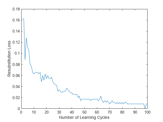
In general, as the number of decision trees in the trained classification ensemble increases, the resubstitution loss decreases.

A decrease in resubstitution loss might indicate that the software trained the ensemble sensibly. However, you cannot infer the predictive power of the ensemble by this decrease. To measure the predictive power of an ensemble, estimate the generalization error by:

  1. Randomly partitioning the data into training and cross-validation sets. Do this by specifying 'holdout',holdoutProportion when you train the ensemble using fitensemble.

  2. Passing the trained ensemble to kfoldLoss, which estimates the generalization error.

Use a trained, boosted regression tree ensemble to predict the fuel economy of a car. Choose the number of cylinders, volume displaced by the cylinders, horsepower, and weight as predictors. Then, train an ensemble using fewer predictors and compare its in-sample predictive accuracy against the first ensemble.

Load the carsmall data set. Store the training data in a table.

load carsmall
Tbl = table(Cylinders,Displacement,Horsepower,Weight,MPG);

Specify a regression tree template that uses surrogate splits to improve predictive accuracy in the presence of NaN values.

t = templateTree('Surrogate','On');

Train the regression tree ensemble using LSBoost and 100 learning cycles.

Mdl1 = fitensemble(Tbl,'MPG','LSBoost',100,t);

Mdl1 is a trained RegressionEnsemble regression ensemble. Because MPG is a variable in the MATLAB® Workspace, you can obtain the same result by entering

Mdl1 = fitensemble(Tbl,MPG,'LSBoost',100,t);

Use the trained regression ensemble to predict the fuel economy for a four-cylinder car with a 200-cubic inch displacement, 150 horsepower, and weighing 3000 lbs.

predMPG = predict(Mdl1,[4 200 150 3000])
predMPG = 22.8462

The average fuel economy of a car with these specifications is 21.78 mpg.

Train a new ensemble using all predictors in Tbl except Displacement.

formula = 'MPG ~ Cylinders + Horsepower + Weight';
Mdl2 = fitensemble(Tbl,formula,'LSBoost',100,t);

Compare the resubstitution MSEs between Mdl1 and Mdl2.

mse1 = resubLoss(Mdl1)
mse1 = 6.4721
mse2 = resubLoss(Mdl2)
mse2 = 7.8599

The in-sample MSE for the ensemble that trains on all predictors is lower.

Estimate the generalization error of a trained, boosting classification ensemble of decision trees.

Load the ionosphere data set.

load ionosphere;

Train a decision tree ensemble using AdaBoostM1, 100 learning cycles, and half of the data chosen randomly. The software validates the algorithm using the remaining half.

rng(2); % For reproducibility
ClassTreeEns = fitensemble(X,Y,'AdaBoostM1',100,'Tree',...
    'Holdout',0.5);

ClassTreeEns is a trained ClassificationEnsemble ensemble classifier.

Determine the cumulative generalization error, i.e., the cumulative misclassification error of the labels in the validation data).

genError = kfoldLoss(ClassTreeEns,'Mode','Cumulative');

genError is a 100-by-1 vector, where element k contains the generalization error after the first k learning cycles.

Plot the generalization error over the number of learning cycles.

plot(genError);
xlabel('Number of Learning Cycles');
ylabel('Generalization Error');

Figure contains an axes object. The axes object with xlabel Number of Learning Cycles, ylabel Generalization Error contains an object of type line.

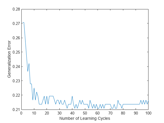
The cumulative generalization error decreases to approximately 7% when 25 weak learners compose the ensemble classifier.

You can control the depth of the trees in an ensemble of decision trees. You can also control the tree depth in an ECOC model containing decision tree binary learners using the MaxNumSplits, MinLeafSize, or MinParentSize name-value pair parameters.

  • When bagging decision trees, fitensemble grows deep decision trees by default. You can grow shallower trees to reduce model complexity or computation time.

  • When boosting decision trees, fitensemble grows stumps (a tree with one split) by default. You can grow deeper trees for better accuracy.

Load the carsmall data set. Specify the variables Acceleration, Displacement, Horsepower, and Weight as predictors, and MPG as the response.

load carsmall
X = [Acceleration Displacement Horsepower Weight];
Y = MPG;

The default values of the tree depth controllers for boosting regression trees are:

  • 1 for MaxNumSplits. This option grows stumps.

  • 5 for MinLeafSize

  • 10 for MinParentSize

To search for the optimal number of splits:

  1. Train a set of ensembles. Exponentially increase the maximum number of splits for subsequent ensembles from stump to at most n - 1 splits, where n is the training sample size. Also, decrease the learning rate for each ensemble from 1 to 0.1.

  2. Cross validate the ensembles.

  3. Estimate the cross-validated mean-squared error (MSE) for each ensemble.

  4. Compare the cross-validated MSEs. The ensemble with the lowest one performs the best, and indicates the optimal maximum number of splits, number of trees, and learning rate for the data set.

Grow and cross validate a deep regression tree and a stump. Specify to use surrogate splits because the data contains missing values. These serve as benchmarks.

MdlDeep = fitrtree(X,Y,'CrossVal','on','MergeLeaves','off',...
    'MinParentSize',1,'Surrogate','on');
MdlStump = fitrtree(X,Y,'MaxNumSplits',1,'CrossVal','on','Surrogate','on');

Train the boosting ensembles using 150 regression trees. Cross validate the ensemble using 5-fold cross validation. Vary the maximum number of splits using the values in the sequence {20,21,...,2m}, where m is such that 2m is no greater than n - 1, where n is the training sample size. For each variant, adjust the learning rate to each value in the set {0.1, 0.25, 0.5, 1};

n = size(X,1);
m = floor(log2(n - 1));
lr = [0.1 0.25 0.5 1];
maxNumSplits = 2.^(0:m);
numTrees = 150;
Mdl = cell(numel(maxNumSplits),numel(lr));
rng(1); % For reproducibility
for k = 1:numel(lr);
    for j = 1:numel(maxNumSplits);
        t = templateTree('MaxNumSplits',maxNumSplits(j),'Surrogate','on');
        Mdl{j,k} = fitensemble(X,Y,'LSBoost',numTrees,t,...
            'Type','regression','KFold',5,'LearnRate',lr(k));
    end;
end;

Compute the cross-validated MSE for each ensemble.

kflAll = @(x)kfoldLoss(x,'Mode','cumulative');
errorCell = cellfun(kflAll,Mdl,'Uniform',false);
error = reshape(cell2mat(errorCell),[numTrees numel(maxNumSplits) numel(lr)]);
errorDeep = kfoldLoss(MdlDeep);
errorStump = kfoldLoss(MdlStump);

Plot how the cross-validated MSE behaves as the number of trees in the ensemble increases for a few of the ensembles, the deep tree, and the stump. Plot the curves with respect to learning rate in the same plot, and plot separate plots for varying tree complexities. Choose a subset of tree complexity levels.

mnsPlot = [1 round(numel(maxNumSplits)/2) numel(maxNumSplits)];
figure;
for k = 1:3;
    subplot(2,2,k);
    plot(squeeze(error(:,mnsPlot(k),:)),'LineWidth',2);
    axis tight;
    hold on;
    h = gca;
    plot(h.XLim,[errorDeep errorDeep],'-.b','LineWidth',2);
    plot(h.XLim,[errorStump errorStump],'-.r','LineWidth',2);
    plot(h.XLim,min(min(error(:,mnsPlot(k),:))).*[1 1],'--k');
    h.YLim = [10 50];    
    xlabel 'Number of trees';
    ylabel 'Cross-validated MSE';
    title(sprintf('MaxNumSplits = %0.3g', maxNumSplits(mnsPlot(k))));
    hold off;
end;
hL = legend([cellstr(num2str(lr','Learning Rate = %0.2f'));...
        'Deep Tree';'Stump';'Min. MSE']);
hL.Position(1) = 0.6;

Figure contains 3 axes objects. Axes object 1 with title MaxNumSplits = 1, xlabel Number of trees, ylabel Cross-validated MSE contains 7 objects of type line. Axes object 2 with title MaxNumSplits = 8, xlabel Number of trees, ylabel Cross-validated MSE contains 7 objects of type line. Axes object 3 with title MaxNumSplits = 64, xlabel Number of trees, ylabel Cross-validated MSE contains 7 objects of type line. These objects represent Learning Rate = 0.10, Learning Rate = 0.25, Learning Rate = 0.50, Learning Rate = 1.00, Deep Tree, Stump, Min. MSE.

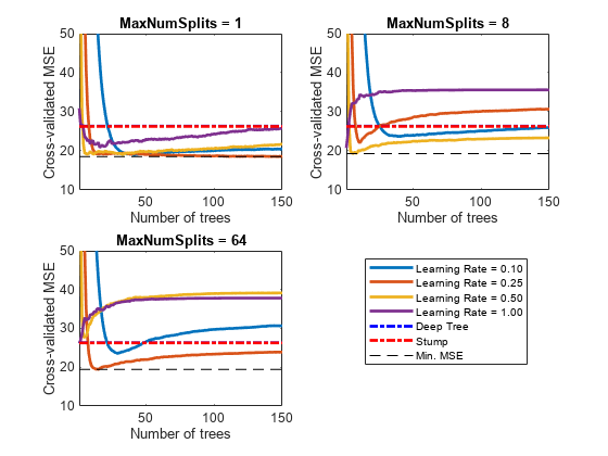
Each curve contains a minimum cross-validated MSE occurring at the optimal number of trees in the ensemble.

Identify the maximum number of splits, number of trees, and learning rate that yields the lowest MSE overall.

[minErr,minErrIdxLin] = min(error(:));
[idxNumTrees,idxMNS,idxLR] = ind2sub(size(error),minErrIdxLin);

fprintf('\nMin. MSE = %0.5f',minErr)
Min. MSE = 18.42979
fprintf('\nOptimal Parameter Values:\nNum. Trees = %d',idxNumTrees);
Optimal Parameter Values:
Num. Trees = 1
fprintf('\nMaxNumSplits = %d\nLearning Rate = %0.2f\n',...
    maxNumSplits(idxMNS),lr(idxLR))
MaxNumSplits = 4
Learning Rate = 1.00

For a different approach to optimizing this ensemble, see Optimize a Boosted Regression Ensemble.

Input Arguments

collapse all

Sample data used to train the model, specified as a table. Each row of Tbl corresponds to one observation, and each column corresponds to one predictor variable. Tbl can contain one additional column for the response variable. Multicolumn variables and cell arrays other than cell arrays of character vectors are not allowed.

  • If Tbl contains the response variable and you want to use all remaining variables as predictors, then specify the response variable using ResponseVarName.

  • If Tbl contains the response variable, and you want to use a subset of the remaining variables only as predictors, then specify a formula using formula.

  • If Tbl does not contain the response variable, then specify the response data using Y. The length of response variable and the number of rows of Tbl must be equal.

Note

To save memory and execution time, supply X and Y instead of Tbl.

Data Types: table

Response variable name, specified as the name of the response variable in Tbl.

You must specify ResponseVarName as a character vector or string scalar. For example, if Tbl.Y is the response variable, then specify ResponseVarName as 'Y'. Otherwise, fitensemble treats all columns of Tbl as predictor variables.

The response variable must be a categorical, character, or string array, a logical or numeric vector, or cell array of character vectors. If the response variable is a character array, then each element must correspond to one row of the array.

For classification, you can specify the order of the classes using the ClassNames name-value pair argument. Otherwise, fitensemble determines the class order, and stores it in the Mdl.ClassNames.

Data Types: char | string

Explanatory model of the response variable and a subset of the predictor variables, specified as a character vector or string scalar in the form "Y~x1+x2+x3". In this form, Y represents the response variable, and x1, x2, and x3 represent the predictor variables.

To specify a subset of variables in Tbl as predictors for training the model, use a formula. If you specify a formula, then the software does not use any variables in Tbl that do not appear in formula.

The variable names in the formula must be both variable names in Tbl (Tbl.Properties.VariableNames) and valid MATLAB® identifiers. You can verify the variable names in Tbl by using the isvarname function. If the variable names are not valid, then you can convert them by using the matlab.lang.makeValidName function.

Data Types: char | string

Predictor data, specified as numeric matrix.

Each row corresponds to one observation, and each column corresponds to one predictor variable.

The length of Y and the number of rows of X must be equal.

To specify the names of the predictors in the order of their appearance in X, use the PredictorNames name-value pair argument.

Data Types: single | double

Response data, specified as a categorical, character, or string array, a logical or numeric vector, or a cell array of character vectors. Each entry in Y is the response to or label for the observation in the corresponding row of X or Tbl. The length of Y and the number of rows of X or Tbl must be equal. If the response variable is a character array, then each element must correspond to one row of the array.

  • For classification, Y can be any of the supported data types. You can specify the order of the classes using the ClassNames name-value pair argument. Otherwise, fitensemble determines the class order, and stores it in the Mdl.ClassNames.

  • For regression, Y must be a numeric column vector.

Data Types: categorical | char | string | logical | single | double | cell

Ensemble aggregation method, specified as one of the method names in this list.

  • For classification with two classes:

    • 'AdaBoostM1'

    • 'LogitBoost'

    • 'GentleBoost'

    • 'RobustBoost' (requires Optimization Toolbox™)

    • 'LPBoost' (requires Optimization Toolbox)

    • 'TotalBoost' (requires Optimization Toolbox)

    • 'RUSBoost'

    • 'Subspace'

    • 'Bag'

  • For classification with three or more classes:

    • 'AdaBoostM2'

    • 'LPBoost' (requires Optimization Toolbox)

    • 'TotalBoost' (requires Optimization Toolbox)

    • 'RUSBoost'

    • 'Subspace'

    • 'Bag'

  • For regression:

    • 'LSBoost'

    • 'Bag'

If you specify 'Method','Bag', then specify the problem type using the Type name-value pair argument, because you can specify 'Bag' for classification and regression problems.

For details about ensemble aggregation algorithms and examples, see Ensemble Algorithms and Choose an Applicable Ensemble Aggregation Method.

Number of ensemble learning cycles, specified as a positive integer or 'AllPredictorCombinations'.

  • If you specify a positive integer, then, at every learning cycle, the software trains one weak learner for every template object in Learners. Consequently, the software trains NLearn*numel(Learners) learners.

  • If you specify 'AllPredictorCombinations', then set Method to 'Subspace' and specify one learner only in Learners. With these settings, the software trains learners for all possible combinations of predictors taken NPredToSample at a time. Consequently, the software trains nchoosek(size(X,2),NPredToSample) learners.

The software composes the ensemble using all trained learners and stores them in Mdl.Trained.

For more details, see Tips.

Data Types: single | double | char | string

Weak learners to use in the ensemble, specified as a weak-learner name, weak-learner template object, or cell array of weak-learner template objects.

Weak LearnerWeak-Learner NameTemplate Object Creation FunctionMethod Settings
Discriminant analysis'Discriminant'templateDiscriminantRecommended for 'Subspace'
k nearest neighbors'KNN'templateKNNFor 'Subspace' only
Decision tree'Tree'templateTreeAll methods except 'Subspace'

For more details, see NLearn and Tips.

Example: For an ensemble composed of two types of classification trees, supply {t1 t2}, where t1 and t2 are classification tree templates.

Name-Value Arguments

Specify optional pairs of arguments as Name1=Value1,...,NameN=ValueN, where Name is the argument name and Value is the corresponding value. Name-value arguments must appear after other arguments, but the order of the pairs does not matter.

Before R2021a, use commas to separate each name and value, and enclose Name in quotes.

Example: 'CrossVal','on','LearnRate',0.05 specifies to implement 10-fold cross-validation and to use 0.05 as the learning rate.

General Ensemble Options

collapse all

Categorical predictors list, specified as one of the values in this table.

ValueDescription
Vector of positive integers

Each entry in the vector is an index value indicating that the corresponding predictor is categorical. The index values are between 1 and p, where p is the number of predictors used to train the model.

If fitensemble uses a subset of input variables as predictors, then the function indexes the predictors using only the subset. The CategoricalPredictors values do not count the response variable, observation weights variable, or any other variables that the function does not use.

Logical vector

A true entry means that the corresponding predictor is categorical. The length of the vector is p.

Character matrixEach row of the matrix is the name of a predictor variable. The names must match the entries in PredictorNames. Pad the names with extra blanks so each row of the character matrix has the same length.
String array or cell array of character vectorsEach element in the array is the name of a predictor variable. The names must match the entries in PredictorNames.
"all"All predictors are categorical.

Specification of 'CategoricalPredictors' is appropriate if:

  • 'Learners' specifies tree learners.

  • 'Learners' specifies k-nearest learners where all predictors are categorical.

Each learner identifies and treats categorical predictors in the same way as the fitting function corresponding to the learner. See 'CategoricalPredictors' of fitcknn for k-nearest learners and 'CategoricalPredictors' of fitctree for tree learners.

Example: 'CategoricalPredictors','all'

Data Types: single | double | logical | char | string | cell

Printout frequency, specified as a positive integer or "off".

To track the number of weak learners or folds that fitensemble trained so far, specify a positive integer. That is, if you specify the positive integer m:

  • Without also specifying any cross-validation option (for example, CrossVal), then fitensemble displays a message to the command line every time it completes training m weak learners.

  • And a cross-validation option, then fitensemble displays a message to the command line every time it finishes training m folds.

If you specify "off", then fitensemble does not display a message when it completes training weak learners.

Tip

For fastest training of some boosted decision trees, set NPrint to the default value "off". This tip holds when the classification Method is "AdaBoostM1", "AdaBoostM2", "GentleBoost", or "LogitBoost", or when the regression Method is "LSBoost".

Example: NPrint=5

Data Types: single | double | char | string

Predictor variable names, specified as a string array of unique names or cell array of unique character vectors. The functionality of PredictorNames depends on the way you supply the training data.

  • If you supply X and Y, then you can use PredictorNames to assign names to the predictor variables in X.

    • The order of the names in PredictorNames must correspond to the column order of X. That is, PredictorNames{1} is the name of X(:,1), PredictorNames{2} is the name of X(:,2), and so on. Also, size(X,2) and numel(PredictorNames) must be equal.

    • By default, PredictorNames is {'x1','x2',...}.

  • If you supply Tbl, then you can use PredictorNames to choose which predictor variables to use in training. That is, fitensemble uses only the predictor variables in PredictorNames and the response variable during training.

    • PredictorNames must be a subset of Tbl.Properties.VariableNames and cannot include the name of the response variable.

    • By default, PredictorNames contains the names of all predictor variables.

    • A good practice is to specify the predictors for training using either PredictorNames or formula, but not both.

Example: "PredictorNames",["SepalLength","SepalWidth","PetalLength","PetalWidth"]

Data Types: string | cell

Response variable name, specified as a character vector or string scalar.

  • If you supply Y, then you can use ResponseName to specify a name for the response variable.

  • If you supply ResponseVarName or formula, then you cannot use ResponseName.

Example: "ResponseName","response"

Data Types: char | string

Supervised learning type, specified as the comma-separated pair consisting of 'Type' and 'classification' or 'regression'.

  • If Method is 'bag', then the supervised learning type is ambiguous. Therefore, specify Type when bagging.

  • Otherwise, the value of Method determines the supervised learning type.

Example: 'Type','classification'

Cross-Validation Options

collapse all

Cross-validation flag, specified as the comma-separated pair consisting of 'Crossval' and 'on' or 'off'.

If you specify 'on', then the software implements 10-fold cross-validation.

To override this cross-validation setting, use one of these name-value pair arguments: CVPartition, Holdout, KFold, or Leaveout. To create a cross-validated model, you can use one cross-validation name-value pair argument at a time only.

Alternatively, cross-validate later by passing Mdl to crossval or crossval.

Example: 'Crossval','on'

Cross-validation partition, specified as a cvpartition object that specifies the type of cross-validation and the indexing for the training and validation sets.

To create a cross-validated model, you can specify only one of these four name-value arguments: CVPartition, Holdout, KFold, or Leaveout.

Example: Suppose you create a random partition for 5-fold cross-validation on 500 observations by using cvp = cvpartition(500,KFold=5). Then, you can specify the cross-validation partition by setting CVPartition=cvp.

Fraction of the data used for holdout validation, specified as a scalar value in the range [0,1]. If you specify Holdout=p, then the software completes these steps:

  1. Randomly select and reserve p*100% of the data as validation data, and train the model using the rest of the data.

  2. Store the compact trained model in the Trained property of the cross-validated model.

To create a cross-validated model, you can specify only one of these four name-value arguments: CVPartition, Holdout, KFold, or Leaveout.

Example: Holdout=0.1

Data Types: double | single

Number of folds to use in the cross-validated model, specified as a positive integer value greater than 1. If you specify KFold=k, then the software completes these steps:

  1. Randomly partition the data into k sets.

  2. For each set, reserve the set as validation data, and train the model using the other k – 1 sets.

  3. Store the k compact trained models in a k-by-1 cell vector in the Trained property of the cross-validated model.

To create a cross-validated model, you can specify only one of these four name-value arguments: CVPartition, Holdout, KFold, or Leaveout.

Example: KFold=5

Data Types: single | double

Leave-one-out cross-validation flag, specified as "on" or "off". If you specify Leaveout="on", then for each of the n observations (where n is the number of observations, excluding missing observations, specified in the NumObservations property of the model), the software completes these steps:

  1. Reserve the one observation as validation data, and train the model using the other n – 1 observations.

  2. Store the n compact trained models in an n-by-1 cell vector in the Trained property of the cross-validated model.

To create a cross-validated model, you can specify only one of these four name-value arguments: CVPartition, Holdout, KFold, or Leaveout.

Example: Leaveout="on"

Data Types: char | string

Other Classification or Regression Options

collapse all

Names of classes to use for training, specified as a categorical, character, or string array; a logical or numeric vector; or a cell array of character vectors. ClassNames must have the same data type as the response variable in Tbl or Y.

If ClassNames is a character array, then each element must correspond to one row of the array.

Use ClassNames to:

  • Specify the order of the classes during training.

  • Specify the order of any input or output argument dimension that corresponds to the class order. For example, use ClassNames to specify the order of the dimensions of Cost or the column order of classification scores returned by predict.

  • Select a subset of classes for training. For example, suppose that the set of all distinct class names in Y is ["a","b","c"]. To train the model using observations from classes "a" and "c" only, specify "ClassNames",["a","c"].

The default value for ClassNames is the set of all distinct class names in the response variable in Tbl or Y.

Example: "ClassNames",["b","g"]

Data Types: categorical | char | string | logical | single | double | cell

Misclassification cost, specified as the comma-separated pair consisting of 'Cost' and a square matrix or structure. If you specify:

  • The square matrix Cost, then Cost(i,j) is the cost of classifying a point into class j if its true class is i. That is, the rows correspond to the true class and the columns correspond to the predicted class. To specify the class order for the corresponding rows and columns of Cost, also specify the ClassNames name-value pair argument.

  • The structure S, then it must have two fields:

    • S.ClassNames, which contains the class names as a variable of the same data type as Y

    • S.ClassificationCosts, which contains the cost matrix with rows and columns ordered as in S.ClassNames

The default is ones(K) - eye(K), where K is the number of distinct classes.

fitensemble uses Cost to adjust the prior class probabilities specified in Prior. Then, fitensemble uses the adjusted prior probabilities for training.

Example: 'Cost',[0 1 2 ; 1 0 2; 2 2 0]

Data Types: double | single | struct

Prior probabilities for each class, specified as the comma-separated pair consisting of 'Prior' and a value in this table.

ValueDescription
'empirical'The class prior probabilities are the class relative frequencies in Y.
'uniform'All class prior probabilities are equal to 1/K, where K is the number of classes.
numeric vectorEach element is a class prior probability. Order the elements according to Mdl.ClassNames or specify the order using the ClassNames name-value pair argument. The software normalizes the elements such that they sum to 1.
structure array

A structure S with two fields:

  • S.ClassNames contains the class names as a variable of the same type as Y.

  • S.ClassProbs contains a vector of corresponding prior probabilities. The software normalizes the elements such that they sum to 1.

fitensemble normalizes the prior probabilities in Prior to sum to 1.

Example: struct('ClassNames',{{'setosa','versicolor','virginica'}},'ClassProbs',1:3)

Data Types: char | string | double | single | struct

Observation weights, specified as the comma-separated pair consisting of 'Weights' and a numeric vector of positive values or name of a variable in Tbl. The software weighs the observations in each row of X or Tbl with the corresponding value in Weights. The size of Weights must equal the number of rows of X or Tbl.

If you specify the input data as a table Tbl, then Weights can be the name of a variable in Tbl that contains a numeric vector. In this case, you must specify Weights as a character vector or string scalar. For example, if the weights vector W is stored as Tbl.W, then specify it as 'W'. Otherwise, the software treats all columns of Tbl, including W, as predictors or the response when training the model.

The software normalizes Weights to sum up to the value of the prior probability in the respective class.

By default, Weights is ones(n,1), where n is the number of observations in X or Tbl.

Data Types: double | single | char | string

Sampling Options for Boosting Methods and Bagging

collapse all

Fraction of the training set to resample for every weak learner, specified as a positive scalar in (0,1]. To use 'FResample', set Resample to 'on'.

Example: 'FResample',0.75

Data Types: single | double

Flag indicating sampling with replacement, specified as the comma-separated pair consisting of 'Replace' and 'off' or 'on'.

  • For 'on', the software samples the training observations with replacement.

  • For 'off', the software samples the training observations without replacement. If you set Resample to 'on', then the software samples training observations assuming uniform weights. If you also specify a boosting method, then the software boosts by reweighting observations.

Unless you set Method to 'bag' or set Resample to 'on', Replace has no effect.

Example: 'Replace','off'

Flag indicating to resample, specified as the comma-separated pair consisting of 'Resample' and 'off' or 'on'.

  • If Method is a boosting method, then:

    • 'Resample','on' specifies to sample training observations using updated weights as the multinomial sampling probabilities.

    • 'Resample','off'(default) specifies to reweight observations at every learning iteration.

  • If Method is 'bag', then 'Resample' must be 'on'. The software resamples a fraction of the training observations (see FResample) with or without replacement (see Replace).

If you specify to resample using Resample, then it is good practice to resample to entire data set. That is, use the default setting of 1 for FResample.

AdaBoostM1, AdaBoostM2, LogitBoost, GentleBoost, and LSBoost Method Options

collapse all

Learning rate for shrinkage, specified as the comma-separated pair consisting of 'LearnRate' and a numeric scalar in the interval (0,1].

To train an ensemble using shrinkage, set LearnRate to a value less than 1, for example, 0.1 is a popular choice. Training an ensemble using shrinkage requires more learning iterations, but often achieves better accuracy.

Example: 'LearnRate',0.1

Data Types: single | double

RUSBoost Method Options

collapse all

Learning rate for shrinkage, specified as the comma-separated pair consisting of 'LearnRate' and a numeric scalar in the interval (0,1].

To train an ensemble using shrinkage, set LearnRate to a value less than 1, for example, 0.1 is a popular choice. Training an ensemble using shrinkage requires more learning iterations, but often achieves better accuracy.

Example: 'LearnRate',0.1

Data Types: single | double

Sampling proportion with respect to the lowest-represented class, specified as the comma-separated pair consisting of 'RatioToSmallest' and a numeric scalar or numeric vector of positive values with length equal to the number of distinct classes in the training data.

Suppose that there are K classes in the training data and the lowest-represented class has m observations in the training data.

  • If you specify the positive numeric scalar s, then fitensemble samples s*m observations from each class, that is, it uses the same sampling proportion for each class. For more details, see Algorithms.

  • If you specify the numeric vector [s1,s2,...,sK], then fitensemble samples si*m observations from class i, i = 1,...,K. The elements of RatioToSmallest correspond to the order of the class names specified using ClassNames (see Tips).

The default value is ones(K,1), which specifies to sample m observations from each class.

Example: 'RatioToSmallest',[2,1]

Data Types: single | double

LPBoost and TotalBoost Method Options

collapse all

Margin precision to control convergence speed, specified as the comma-separated pair consisting of 'MarginPrecision' and a numeric scalar in the interval [0,1]. MarginPrecision affects the number of boosting iterations required for convergence.

Tip

To train an ensemble using many learners, specify a small value for MarginPrecision. For training using a few learners, specify a large value.

Example: 'MarginPrecision',0.5

Data Types: single | double

RobustBoost Method Options

collapse all

Target classification error, specified as the comma-separated pair consisting of 'RobustErrorGoal' and a nonnegative numeric scalar. The upper bound on possible values depends on the values of RobustMarginSigma and RobustMaxMargin. However, the upper bound cannot exceed 1.

Tip

For a particular training set, usually there is an optimal range for RobustErrorGoal. If you set it too low or too high, then the software can produce a model with poor classification accuracy. Try cross-validating to search for the appropriate value.

Example: 'RobustErrorGoal',0.05

Data Types: single | double

Classification margin distribution spread over the training data, specified as the comma-separated pair consisting of 'RobustMarginSigma' and a positive numeric scalar. Before specifying RobustMarginSigma, consult the literature on RobustBoost, for example, [19].

Example: 'RobustMarginSigma',0.5

Data Types: single | double

Maximal classification margin in the training data, specified as the comma-separated pair consisting of 'RobustMaxMargin' and a nonnegative numeric scalar. The software minimizes the number of observations in the training data having classification margins below RobustMaxMargin.

Example: 'RobustMaxMargin',1

Data Types: single | double

Random Subspace Method Options

collapse all

Number of predictors to sample for each random subspace learner, specified as the comma-separated pair consisting of 'NPredToSample' and a positive integer in the interval 1,...,p, where p is the number of predictor variables (size(X,2) or size(Tbl,2)).

Data Types: single | double

Output Arguments

collapse all

Trained ensemble model, returned as one of the model objects in this table.

Model ObjectType SettingSpecify Any Cross-Validation Options?Method SettingResample Setting
ClassificationBaggedEnsemble'classification'No'Bag''on'
ClassificationEnsemble'classification'NoAny ensemble-aggregation method for classification'off'
ClassificationPartitionedEnsemble'classification'YesAny classification ensemble-aggregation method'off' or 'on'
RegressionBaggedEnsemble'regression'No'Bag''on'
RegressionEnsemble'regression'No'LSBoost''off'
RegressionPartitionedEnsemble'regression'Yes'LSBoost' or 'Bag''off' or 'on'

The name-value pair arguments that control cross-validation are CrossVal, Holdout, KFold, Leaveout, and CVPartition.

To reference properties of Mdl, use dot notation. For example, to access or display the cell vector of weak learner model objects for an ensemble that has not been cross-validated, enter Mdl.Trained at the command line.

Tips

  • NLearn can vary from a few dozen to a few thousand. Usually, an ensemble with good predictive power requires from a few hundred to a few thousand weak learners. However, you do not have to train an ensemble for that many cycles at once. You can start by growing a few dozen learners, inspect the ensemble performance and then, if necessary, train more weak learners using resume for classification problems, or resume for regression problems.

  • Ensemble performance depends on the ensemble setting and the setting of the weak learners. That is, if you specify weak learners with default parameters, then the ensemble can perform poorly. Therefore, like ensemble settings, it is good practice to adjust the parameters of the weak learners using templates, and to choose values that minimize generalization error.

  • If you specify to resample using Resample, then it is good practice to resample to entire data set. That is, use the default setting of 1 for FResample.

  • In classification problems (that is, Type is 'classification'):

    • If the ensemble-aggregation method (Method) is 'bag' and:

      • The misclassification cost (Cost) is highly imbalanced, then, for in-bag samples, the software oversamples unique observations from the class that has a large penalty.

      • The class prior probabilities (Prior) are highly skewed, the software oversamples unique observations from the class that has a large prior probability.

      For smaller sample sizes, these combinations can result in a low relative frequency of out-of-bag observations from the class that has a large penalty or prior probability. Consequently, the estimated out-of-bag error is highly variable and it can be difficult to interpret. To avoid large estimated out-of-bag error variances, particularly for small sample sizes, set a more balanced misclassification cost matrix using Cost or a less skewed prior probability vector using Prior.

    • Because the order of some input and output arguments correspond to the distinct classes in the training data, it is good practice to specify the class order using the ClassNames name-value pair argument.

      • To determine the class order quickly, remove all observations from the training data that are unclassified (that is, have a missing label), obtain and display an array of all the distinct classes, and then specify the array for ClassNames. For example, suppose the response variable (Y) is a cell array of labels. This code specifies the class order in the variable classNames.

        Ycat = categorical(Y);
        classNames = categories(Ycat)
        categorical assigns <undefined> to unclassified observations and categories excludes <undefined> from its output. Therefore, if you use this code for cell arrays of labels or similar code for categorical arrays, then you do not have to remove observations with missing labels to obtain a list of the distinct classes.

      • To specify that the class order from lowest-represented label to most-represented, then quickly determine the class order (as in the previous bullet), but arrange the classes in the list by frequency before passing the list to ClassNames. Following from the previous example, this code specifies the class order from lowest- to most-represented in classNamesLH.

        Ycat = categorical(Y);
        classNames = categories(Ycat);
        freq = countcats(Ycat);
        [~,idx] = sort(freq);
        classNamesLH = classNames(idx);

Algorithms

  • For details of ensemble-aggregation algorithms, see Ensemble Algorithms.

  • If you specify Method to be a boosting algorithm and Learners to be decision trees, then the software grows stumps by default. A decision stump is one root node connected to two terminal, leaf nodes. You can adjust tree depth by specifying the MaxNumSplits, MinLeafSize, and MinParentSize name-value pair arguments using templateTree.

  • fitensemble generates in-bag samples by oversampling classes with large misclassification costs and undersampling classes with small misclassification costs. Consequently, out-of-bag samples have fewer observations from classes with large misclassification costs and more observations from classes with small misclassification costs. If you train a classification ensemble using a small data set and a highly skewed cost matrix, then the number of out-of-bag observations per class can be low. Therefore, the estimated out-of-bag error can have a large variance and can be difficult to interpret. The same phenomenon can occur for classes with large prior probabilities.

  • For the RUSBoost ensemble-aggregation method (Method), the name-value pair argument RatioToSmallest specifies the sampling proportion for each class with respect to the lowest-represented class. For example, suppose that there are two classes in the training data: A and B. A have 100 observations and B have 10 observations. Also, suppose that the lowest-represented class has m observations in the training data.

    • If you set 'RatioToSmallest',2, then s*m = 2*10 = 20. Consequently, fitensemble trains every learner using 20 observations from class A and 20 observations from class B. If you set 'RatioToSmallest',[2 2], then you obtain the same result.

    • If you set 'RatioToSmallest',[2,1], then s1*m = 2*10 = 20 and s2*m = 1*10 = 10. Consequently, fitensemble trains every learner using 20 observations from class A and 10 observations from class B.

  • For ensembles of decision trees, and for dual-core systems and above, fitensemble parallelizes training using Intel® Threading Building Blocks (TBB). For details on Intel TBB, see https://www.intel.com/content/www/us/en/developer/tools/oneapi/onetbb.html.

References

[1] Breiman, L. “Bagging Predictors.” Machine Learning. Vol. 26, pp. 123–140, 1996.

[2] Breiman, L. “Random Forests.” Machine Learning. Vol. 45, pp. 5–32, 2001.

[3] Freund, Y. “A more robust boosting algorithm.” arXiv:0905.2138v1, 2009.

[4] Freund, Y. and R. E. Schapire. “A Decision-Theoretic Generalization of On-Line Learning and an Application to Boosting.” J. of Computer and System Sciences, Vol. 55, pp. 119–139, 1997.

[5] Friedman, J. “Greedy function approximation: A gradient boosting machine.” Annals of Statistics, Vol. 29, No. 5, pp. 1189–1232, 2001.

[6] Friedman, J., T. Hastie, and R. Tibshirani. “Additive logistic regression: A statistical view of boosting.” Annals of Statistics, Vol. 28, No. 2, pp. 337–407, 2000.

[7] Hastie, T., R. Tibshirani, and J. Friedman. The Elements of Statistical Learning section edition, Springer, New York, 2008.

[8] Ho, T. K. “The random subspace method for constructing decision forests.” IEEE Transactions on Pattern Analysis and Machine Intelligence, Vol. 20, No. 8, pp. 832–844, 1998.

[9] Schapire, R. E., Y. Freund, P. Bartlett, and W.S. Lee. “Boosting the margin: A new explanation for the effectiveness of voting methods.” Annals of Statistics, Vol. 26, No. 5, pp. 1651–1686, 1998.

[10] Seiffert, C., T. Khoshgoftaar, J. Hulse, and A. Napolitano. “RUSBoost: Improving classification performance when training data is skewed.” 19th International Conference on Pattern Recognition, pp. 1–4, 2008.

[11] Warmuth, M., J. Liao, and G. Ratsch. “Totally corrective boosting algorithms that maximize the margin.” Proc. 23rd Int’l. Conf. on Machine Learning, ACM, New York, pp. 1001–1008, 2006.

Extended Capabilities

Version History

Introduced in R2011a