fitrgp

Fit a Gaussian process regression (GPR) model

Syntax

Mdl = fitrgp(Tbl,ResponseVarName)

Mdl = fitrgp(Tbl,formula)

Mdl = fitrgp(Tbl,y)

Mdl = fitrgp(X,y)

Mdl = fitrgp(___,Name=Value)

[Mdl,AggregateOptimizationResults] = fitrgp(___)

Description

Mdl = fitrgp(Tbl,ResponseVarName) returns a Gaussian process regression (GPR) model trained using the sample data in Tbl, where ResponseVarName is the name of the response variable in Tbl.

Mdl = fitrgp(Tbl,formula) returns a Gaussian process regression (GPR) model, trained using the sample data in Tbl, for the predictor variables and response variables identified by formula.

Mdl = fitrgp(Tbl,y) returns a GPR model for the predictors in table Tbl and continuous response vector y.

Mdl = fitrgp(X,y) returns a GPR model for predictors X and continuous response vector y.

Mdl = fitrgp(___,Name=Value) returns a GPR model for any of the input arguments in the previous syntaxes, with additional options specified by one or more name-value arguments.

For example, you can specify the fitting method, the prediction method, the covariance function, or the active set selection method. You can also train a cross-validated model.

Mdl is a RegressionGP object. For object functions and properties of this object, see RegressionGP.

If you train a cross-validated model, then Mdl is a RegressionPartitionedGP object. For further analysis on the cross-validated object, use the object functions of the RegressionPartitionedGP object.

[Mdl,AggregateOptimizationResults] = fitrgp(___) also returns AggregateOptimizationResults, which contains hyperparameter optimization results when you specify the OptimizeHyperparameters and HyperparameterOptimizationOptions name-value arguments. You must also specify the ConstraintType and ConstraintBounds options of HyperparameterOptimizationOptions. You can use this syntax to optimize on compact model size instead of cross-validation loss, and to perform a set of multiple optimization problems that have the same options but different constraint bounds.

Examples

Train GPR Model Using Data in Table

This example uses the abalone data [1], [2], from the UCI Machine Learning Repository [3]. Download the data and save it in your current folder with the name abalone.data.

Store the data into a table. Display the first seven rows.

tbl = readtable('abalone.data','Filetype','text',...
     'ReadVariableNames',false);
tbl.Properties.VariableNames = {'Sex','Length','Diameter','Height',...
     'WWeight','SWeight','VWeight','ShWeight','NoShellRings'};
tbl(1:7,:)

ans = 

    Sex    Length    Diameter    Height    WWeight    SWeight    VWeight    ShWeight    NoShellRings
    ___    ______    ________    ______    _______    _______    _______    ________    ____________

    'M'    0.455     0.365       0.095      0.514     0.2245      0.101      0.15       15          
    'M'     0.35     0.265        0.09     0.2255     0.0995     0.0485      0.07        7          
    'F'     0.53      0.42       0.135      0.677     0.2565     0.1415      0.21        9          
    'M'     0.44     0.365       0.125      0.516     0.2155      0.114     0.155       10          
    'I'     0.33     0.255        0.08      0.205     0.0895     0.0395     0.055        7          
    'I'    0.425       0.3       0.095     0.3515      0.141     0.0775      0.12        8          
    'F'     0.53     0.415        0.15     0.7775      0.237     0.1415      0.33       20

The dataset has 4177 observations. The goal is to predict the age of abalone from eight physical measurements. The last variable, number of shell rings shows the age of the abalone. The first predictor is a categorical variable. The last variable in the table is the response variable.

Fit a GPR model using the subset of regressors method for parameter estimation and fully independent conditional method for prediction. Standardize the predictors.

gprMdl = fitrgp(tbl,'NoShellRings','KernelFunction','ardsquaredexponential',...
      'FitMethod','sr','PredictMethod','fic','Standardize',1)

grMdl = 

  RegressionGP
       PredictorNames: {1x8 cell}
         ResponseName: 'Var9'
    ResponseTransform: 'none'
      NumObservations: 4177
       KernelFunction: 'ARDSquaredExponential'
    KernelInformation: [1x1 struct]
        BasisFunction: 'Constant'
                 Beta: 10.9148
                Sigma: 2.0243
    PredictorLocation: [10x1 double]
       PredictorScale: [10x1 double]
                Alpha: [1000x1 double]
     ActiveSetVectors: [1000x10 double]
        PredictMethod: 'FIC'
        ActiveSetSize: 1000
            FitMethod: 'SR'
      ActiveSetMethod: 'Random'
    IsActiveSetVector: [4177x1 logical]
        LogLikelihood: -9.0013e+03
     ActiveSetHistory: [1x1 struct]
       BCDInformation: []

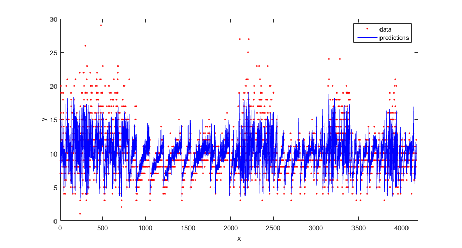
Predict the responses using the trained model.

ypred = resubPredict(gprMdl);

Plot the true response and the predicted responses.

figure();
plot(tbl.NoShellRings,'r.');
hold on
plot(ypred,'b');
xlabel('x');
ylabel('y');
legend({'data','predictions'},'Location','Best');
axis([0 4300 0 30]);
hold off;

Compute the regression loss on the training data (resubstitution loss) for the trained model.

L = resubLoss(gprMdl)

L =

    4.0064

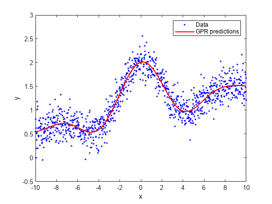
Train GPR Model and Plot Predictions

Generate sample data.

rng(0,'twister'); % For reproducibility
n = 1000;
x = linspace(-10,10,n)';
y = 1 + x*5e-2 + sin(x)./x + 0.2*randn(n,1);

Fit a GPR model using a linear basis function and the exact fitting method to estimate the parameters. Also use the exact prediction method.

gprMdl = fitrgp(x,y,'Basis','linear',...
      'FitMethod','exact','PredictMethod','exact');

Predict the response corresponding to the rows of x (resubstitution predictions) using the trained model.

ypred = resubPredict(gprMdl);

Plot the true response with the predicted values.

plot(x,y,'b.');
hold on;
plot(x,ypred,'r','LineWidth',1.5);
xlabel('x');
ylabel('y');
legend('Data','GPR predictions');
hold off

Impact of Specifying Initial Kernel Parameter Values

Load the sample data.

load('gprdata2.mat')

The data has one predictor variable and continuous response. This is simulated data.

Fit a GPR model using the squared exponential kernel function with default kernel parameters.

gprMdl1 = fitrgp(x,y,'KernelFunction','squaredexponential');

Now, fit a second model, where you specify the initial values for the kernel parameters.

sigma0 = 0.2;
kparams0 = [3.5, 6.2];
gprMdl2 = fitrgp(x,y,'KernelFunction','squaredexponential',...
     'KernelParameters',kparams0,'Sigma',sigma0);

Compute the resubstitution predictions from both models.

ypred1 = resubPredict(gprMdl1);
ypred2 = resubPredict(gprMdl2);

Plot the response predictions from both models and the responses in training data.

figure();
plot(x,y,'r.');
hold on
plot(x,ypred1,'b');
plot(x,ypred2,'g');
xlabel('x');
ylabel('y');
legend({'data','default kernel parameters',...
'kparams0 = [3.5,6.2], sigma0 = 0.2'},...
'Location','Best');
title('Impact of initial kernel parameter values');
hold off

The marginal log likelihood that fitrgp maximizes to estimate GPR parameters has multiple local solutions; the solution that it converges to depends on the initial point. Each local solution corresponds to a particular interpretation of the data. In this example, the solution with the default initial kernel parameters corresponds to a low frequency signal with high noise whereas the second solution with custom initial kernel parameters corresponds to a high frequency signal with low noise.

Use Separate Length Scales for Predictors

Load the sample data.

load('gprdata.mat')

There are six continuous predictor variables. There are 500 observations in the training data set and 100 observations in the test data set. This is simulated data.

Fit a GPR model using the squared exponential kernel function with a separate length scale for each predictor. This covariance function is defined as:

$$k(x_i,x_j|\theta )={\sigma }_f^{2}exp\left[-\frac{1}{2}\sum _{m=1}^d\frac{{(x_{im}-x_{jm})}^2}{{\sigma }_m^2}\right].$$

where $${\sigma }_m$$ represents the length scale for predictor $$m$$, $$m$$ = 1, 2, ..., $$d$$ and $${\sigma }_f$$ is the signal standard deviation. The unconstrained parametrization $$\theta$$ is

$$\begin{array}{l}{\theta }_m=\log {\sigma }_m,form=1,2,...,d\\ {\theta }_{d+1}=\log {\sigma }_f.\end{array}$$

Initialize length scales of the kernel function at 10 and signal and noise standard deviations at the standard deviation of the response.

sigma0 = std(ytrain);
sigmaF0 = sigma0;
d = size(Xtrain,2);
sigmaM0 = 10*ones(d,1);

Fit the GPR model using the initial kernel parameter values. Standardize the predictors in the training data. Use the exact fitting and prediction methods.

gprMdl = fitrgp(Xtrain,ytrain,'Basis','constant','FitMethod','exact',...
'PredictMethod','exact','KernelFunction','ardsquaredexponential',...
'KernelParameters',[sigmaM0;sigmaF0],'Sigma',sigma0,'Standardize',1);

Compute the regression loss on the test data.

L = loss(gprMdl,Xtest,ytest)

L = 
0.6919

Access the kernel information.

gprMdl.KernelInformation

ans = struct with fields:
                    Name: 'ARDSquaredExponential'
        KernelParameters: [7×1 double]
    KernelParameterNames: {7×1 cell}

Display the kernel parameter names. When you use an ARD kernel, the length scale parameters correspond to the expanded predictors. Replace the length scale parameter names with the expanded predictor names.

paramNames = gprMdl.KernelInformation.KernelParameterNames

paramNames = 7×1 cell
    {'LengthScale1'}
    {'LengthScale2'}
    {'LengthScale3'}
    {'LengthScale4'}
    {'LengthScale5'}
    {'LengthScale6'}
    {'SigmaF'      }

paramNames(1:end-1) = gprMdl.ExpandedPredictorNames

paramNames = 7×1 cell
    {'x1'    }
    {'x2'    }
    {'x3'    }
    {'x4'    }
    {'x5'    }
    {'x6'    }
    {'SigmaF'}

Display the kernel parameters.

sigmaM = gprMdl.KernelInformation.KernelParameters(1:end-1,1)

sigmaM = 6×1
104 ×

    0.0004
    0.0007
    0.0004
    4.7605
    0.1018
    0.0056

sigmaF = gprMdl.KernelInformation.KernelParameters(end)

sigmaF = 
28.1720

sigma  = gprMdl.Sigma

sigma = 
0.8162

Plot the log of learned length scales.

figure()
plot((1:d)',log(sigmaM),'ro-');
xlabel('Length scale number');
ylabel('Log of length scale');

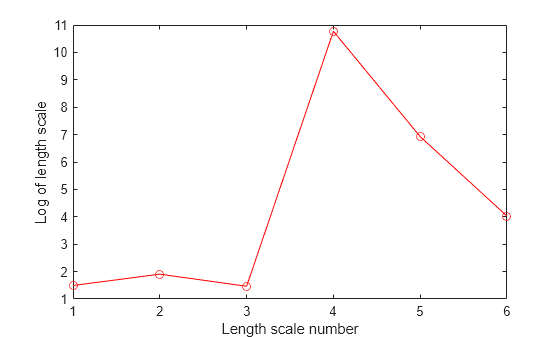
The log of length scale for the 4th and 5th predictor variables are high relative to the others. These predictor variables do not seem to be as influential on the response as the other predictor variables.

Fit the GPR model without using the 4th and 5th variables as the predictor variables.

X = [Xtrain(:,1:3) Xtrain(:,6)];
sigma0 = std(ytrain);
sigmaF0 = sigma0;
d = size(X,2);
sigmaM0 = 10*ones(d,1);

gprMdl = fitrgp(X,ytrain,'Basis','constant','FitMethod','exact',...
'PredictMethod','exact','KernelFunction','ardsquaredexponential',...
'KernelParameters',[sigmaM0;sigmaF0],'Sigma',sigma0,'Standardize',1);

Compute the regression error on the test data.

xtest = [Xtest(:,1:3) Xtest(:,6)];
L = loss(gprMdl,xtest,ytest)

L = 
0.6928

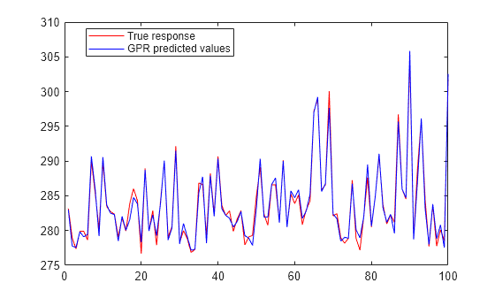
The loss is similar to the one when all variables are used as predictor variables.

Compute the predicted response for the test data.

 ypred = predict(gprMdl,xtest);

Plot the original response along with the fitted values.

figure;
plot(ytest,'r');
hold on;
plot(ypred,'b');
legend('True response','GPR predicted values','Location','Best');
hold off

Optimize GPR Model

Automatically optimize hyperparameters of a GPR model using fitrgp. Compare the fit of the model with the optimized hyperparameter values to the fit of the model with the default hyperparameter values.

Load the gprdata2 data set.

load gprdata2

The simulated data consists of one predictor variable and one continuous response.

Fit a GPR model using the squared exponential kernel function with default kernel parameters.

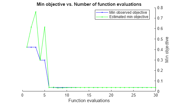
gprMdl1 = fitrgp(x,y,KernelFunction="squaredexponential");

Find hyperparameters that minimize the 5-fold cross-validation loss by using automatic hyperparameter optimization. For reproducibility, set the random seed and use the "expected-improvement-plus" acquisition function.

rng(0,"twister")
hpoOptions = hyperparameterOptimizationOptions(AcquisitionFunctionName="expected-improvement-plus");
gprMdl2 = fitrgp(x,y,KernelFunction="squaredexponential", ...
    OptimizeHyperparameters="auto",HyperparameterOptimizationOptions=hpoOptions);

|=====================================================================================================|
| Iter | Eval   | Objective:  | Objective   | BestSoFar   | BestSoFar   |        Sigma |  Standardize |
|      | result | log(1+loss) | runtime     | (observed)  | (estim.)    |              |              |
|=====================================================================================================|
|    1 | Best   |     0.42258 |      1.5225 |     0.42258 |     0.42258 |       2.7255 |        false |
|    2 | Accept |      1.5061 |      1.9339 |     0.42258 |     0.72573 |    0.0057724 |         true |
|    3 | Accept |      1.6498 |     0.73634 |     0.42258 |     0.44024 |       25.905 |         true |
|    4 | Best   |     0.29824 |      2.1104 |     0.29824 |     0.34769 |    0.0098001 |        false |
|    5 | Accept |     0.29873 |        2.32 |     0.29824 |     0.28958 |   0.00010004 |        false |
|    6 | Accept |     0.29873 |      2.6094 |     0.29824 |     0.29843 |   0.00010043 |        false |
|    7 | Accept |      1.5335 |      1.8128 |     0.29824 |     0.29874 |    0.0010605 |        false |
|    8 | Accept |      1.4588 |      1.6501 |     0.29824 |     0.93331 |     0.015898 |        false |
|    9 | Accept |      2.0988 |     0.86788 |     0.29824 |      1.0628 |       29.197 |        false |
|   10 | Accept |     0.29873 |      2.0644 |     0.29824 |     0.29875 |   0.00010018 |        false |
|   11 | Accept |     0.29839 |      2.0358 |     0.29824 |     0.92386 |    0.0081946 |        false |
|   12 | Accept |      1.0384 |      1.5563 |     0.29824 |      0.9334 |    0.0029634 |        false |
|   13 | Accept |     0.29873 |      2.0199 |     0.29824 |     0.29875 |   0.00010028 |        false |
|   14 | Accept |     0.29873 |      2.0423 |     0.29824 |      0.2985 |   0.00013764 |        false |
|   15 | Accept |     0.42286 |     0.87571 |     0.29824 |     0.29852 |       1.7961 |        false |
|   16 | Accept |      1.0387 |      1.4747 |     0.29824 |     0.29753 |   0.00021994 |        false |
|   17 | Accept |     0.29873 |      1.9232 |     0.29824 |     0.29877 |    0.0001181 |        false |
|   18 | Accept |     0.42357 |        0.79 |     0.29824 |     0.29878 |      0.99648 |        false |
|   19 | Accept |     0.42164 |     0.76652 |     0.29824 |     0.29879 |      0.56592 |        false |
|   20 | Best   |    0.037686 |      1.5945 |    0.037686 |    0.037782 |      0.30638 |        false |
|=====================================================================================================|
| Iter | Eval   | Objective:  | Objective   | BestSoFar   | BestSoFar   |        Sigma |  Standardize |
|      | result | log(1+loss) | runtime     | (observed)  | (estim.)    |              |              |
|=====================================================================================================|
|   21 | Accept |    0.037728 |      1.1352 |    0.037686 |    0.037733 |      0.21519 |        false |
|   22 | Accept |    0.038324 |      1.0433 |    0.037686 |    0.037677 |      0.12756 |        false |
|   23 | Accept |    0.037841 |       1.123 |    0.037686 |    0.037707 |       0.1587 |        false |
|   24 | Accept |     0.04014 |     0.97319 |    0.037686 |     0.03764 |     0.082293 |        false |
|   25 | Accept |    0.039534 |      1.0481 |    0.037686 |    0.037656 |     0.098414 |        false |
|   26 | Accept |    0.037718 |      1.1948 |    0.037686 |    0.037656 |      0.34831 |         true |
|   27 | Accept |     0.42164 |     0.80799 |    0.037686 |    0.037659 |      0.57775 |         true |
|   28 | Accept |    0.037733 |      1.3255 |    0.037686 |    0.037652 |      0.21148 |         true |
|   29 | Accept |    0.039512 |     0.89786 |    0.037686 |    0.037648 |     0.099436 |         true |
|   30 | Accept |     0.28105 |      1.8193 |    0.037686 |    0.037647 |     0.054662 |         true |

__________________________________________________________
Optimization completed.
MaxObjectiveEvaluations of 30 reached.
Total function evaluations: 30
Total elapsed time: 70.1885 seconds
Total objective function evaluation time: 44.075

Best observed feasible point:
     Sigma     Standardize
    _______    ___________

    0.30638       false   

Observed objective function value = 0.037686
Estimated objective function value = 0.037806
Function evaluation time = 1.5945

Best estimated feasible point (according to models):
     Sigma     Standardize
    _______    ___________

    0.21519       false   

Estimated objective function value = 0.037647
Estimated function evaluation time = 1.1122

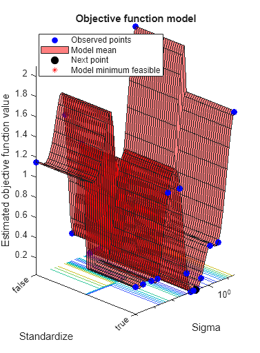
The trained regression model gprMdl2 corresponds to the best estimated feasible point and uses the same hyperparameter values for Sigma and Standardize.

Find the hyperparameter values used to train gprMdl2 by using the bestPoint function. By default, bestPoint uses the same best point criterion used by fitrgp during the hyperparameter optimization ("min-visited-upper-confidence-interval"). In general, fit functions determine the best hyperparameter values based on the "min-visited-upper-confidence-interval" criterion (instead of the "min-observed" criterion) to avoid overfitting to noise in the data set.

bestEstimatedPoint = bestPoint(gprMdl2.HyperparameterOptimizationResults)

bestEstimatedPoint=1×2 table
     Sigma     Standardize
    _______    ___________

    0.21519       false   

Verify that the results match the properties of gprMdl2. Note that the PredictorLocation and PredictorScale properties of a RegressionGP object are nonempty when the GPR model uses standardization.

modelProperties = table(gprMdl2.Sigma, ...
    struct(Mean=gprMdl2.PredictorLocation, ...
    StandardDeviation=gprMdl2.PredictorScale), ...
    VariableNames=["Sigma","Standardize"])

modelProperties=1×2 table
     Sigma     Standardize
    _______    ___________

    0.21519    1×1 struct 

modelProperties.Standardize

ans = struct with fields:
                 Mean: []
    StandardDeviation: []

Visually compare the pre- and post-optimization fits.

ypred1 = resubPredict(gprMdl1);
ypred2 = resubPredict(gprMdl2);

figure
plot(x,y,".")
hold on
plot(x,ypred1)
plot(x,ypred2)
xlabel("x");
ylabel("y");
legend(["Data","Default fit","Optimized fit"], ...
    Location="best")
title("Impact of Optimization")
hold off

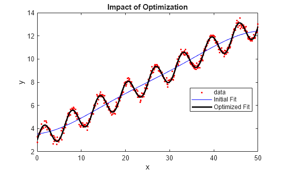
The model with the optimized hyperparameters provides a better fit to the training data.

Train GPR Model Using Cross-Validation

This example uses the abalone data [1], [2], from the UCI Machine Learning Repository [3]. Download the data and save it in your current folder with the name abalone.data.

Store the data into a table. Display the first seven rows.

tbl = readtable('abalone.data','Filetype','text','ReadVariableNames',false);
tbl.Properties.VariableNames = {'Sex','Length','Diameter','Height','WWeight','SWeight','VWeight','ShWeight','NoShellRings'};
tbl(1:7,:)

ans = 

    Sex    Length    Diameter    Height    WWeight    SWeight    VWeight    ShWeight    NoShellRings
    ___    ______    ________    ______    _______    _______    _______    ________    ____________

    'M'    0.455     0.365       0.095      0.514     0.2245      0.101      0.15       15          
    'M'     0.35     0.265        0.09     0.2255     0.0995     0.0485      0.07        7          
    'F'     0.53      0.42       0.135      0.677     0.2565     0.1415      0.21        9          
    'M'     0.44     0.365       0.125      0.516     0.2155      0.114     0.155       10          
    'I'     0.33     0.255        0.08      0.205     0.0895     0.0395     0.055        7          
    'I'    0.425       0.3       0.095     0.3515      0.141     0.0775      0.12        8          
    'F'     0.53     0.415        0.15     0.7775      0.237     0.1415      0.33       20

The dataset has 4177 observations. The goal is to predict the age of abalone from eight physical measurements. The last variable, number of shell rings shows the age of the abalone. The first predictor is a categorical variable. The last variable in the table is the response variable.

Train a cross-validated GPR model using the 25% of the data for validation.

rng('default') % For reproducibility
cvgprMdl = fitrgp(tbl,'NoShellRings','Standardize',1,'Holdout',0.25);

Compute the average loss on folds using models trained on out-of-fold observations.

kfoldLoss(cvgprMdl)

ans =
   4.6409

Predict the responses for out-of-fold data.

ypred = kfoldPredict(cvgprMdl);

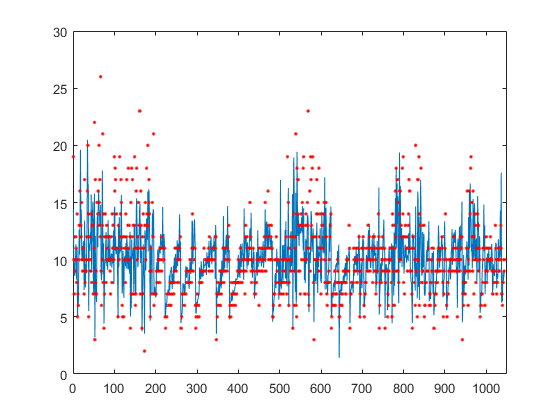
Plot the true responses used for testing and the predictions.

figure();
plot(ypred(cvgprMdl.Partition.test));
hold on;
y = table2array(tbl(:,end));
plot(y(cvgprMdl.Partition.test),'r.');
axis([0 1050 0 30]);
xlabel('x')
ylabel('y')
hold off;

Fit GPR Model Using Custom Kernel Function

Generate the sample data.

rng(0,'twister'); % For reproducibility
n = 1000;
x = linspace(-10,10,n)';
y = 1 + x*5e-2 + sin(x)./x + 0.2*randn(n,1);

Define the squared exponential kernel function as a custom kernel function.

You can compute the squared exponential kernel function as

$$k(x_i,x_j|\theta )={\sigma }_f^2\exp \left(-\frac{1}{2}\frac{(x_i-x_j{)}^T(x_i-x_j)}{{\sigma }_l^2}\right),$$

where $${\sigma }_f$$ is the signal standard deviation, $${\sigma }_l$$ is the length scale. Both $${\sigma }_f$$ and $${\sigma }_l$$ must be greater than zero. This condition can be enforced by the unconstrained parameterization, $${\sigma }_l=\exp (\theta (1))$$ and $${\sigma }_f=\exp (\theta (2))$$, for some unconstrained parameterization vector $$\theta$$.

Hence, you can define the squared exponential kernel function as a custom kernel function as follows:

kfcn = @(XN,XM,theta) (exp(theta(2))^2)*exp(-(pdist2(XN,XM).^2)/(2*exp(theta(1))^2));

Here pdist2(XN,XM).^2 computes the distance matrix.

Fit a GPR model using the custom kernel function, kfcn. Specify the initial values of the kernel parameters (Because you use a custom kernel function, you must provide initial values for the unconstrained parameterization vector, theta).

theta0 = [1.5,0.2];
gprMdl = fitrgp(x,y,'KernelFunction',kfcn,'KernelParameters',theta0);

fitrgp uses analytical derivatives to estimate parameters when using a built-in kernel function, whereas when using a custom kernel function it uses numerical derivatives.

Compute the resubstitution loss for this model.

L = resubLoss(gprMdl)

L = 
0.0391

Fit the GPR model using the built-in squared exponential kernel function option. Specify the initial values of the kernel parameters (Because you use the built-in custom kernel function and specifying initial parameter values, you must provide the initial values for the signal standard deviation and length scale(s) directly).

sigmaL0 = exp(1.5);
sigmaF0 = exp(0.2);
gprMdl2 = fitrgp(x,y,'KernelFunction','squaredexponential','KernelParameters',[sigmaL0,sigmaF0]);

Compute the resubstitution loss for this model.

L2 = resubLoss(gprMdl2)

L2 = 
0.0391

The two loss values are the same as expected.

Specify Initial Step Size for LBFGS Optimization

Train a GPR model on generated data with many predictors. Specify the initial step size for the LBFGS optimizer.

Set the seed and type of the random number generator for reproducibility of the results.

rng(0,'twister'); % For reproducibility 

Generate sample data with 300 observations and 3000 predictors, where the response variable depends on the 4th, 7th, and 13th predictors.

N = 300;
P = 3000;
X = rand(N,P);
y = cos(X(:,7)) + sin(X(:,4).*X(:,13)) + 0.1*randn(N,1);

Set initial values for the kernel parameters.

sigmaL0 = sqrt(P)*ones(P,1); % Length scale for predictors
sigmaF0 = 1; % Signal standard deviation

Set initial noise standard deviation to 1.

sigmaN0 = 1;

Specify 1e-2 as the termination tolerance for the relative gradient norm.

opts = statset('fitrgp');
opts.TolFun = 1e-2;

Fit a GPR model using the initial kernel parameter values, initial noise standard deviation, and an automatic relevance determination (ARD) squared exponential kernel function.

Specify the initial step size as 1 for determining the initial Hessian approximation for an LBFGS optimizer.

gpr = fitrgp(X,y,'KernelFunction','ardsquaredexponential','Verbose',1, ...
    'Optimizer','lbfgs','OptimizerOptions',opts, ...
    'KernelParameters',[sigmaL0;sigmaF0],'Sigma',sigmaN0,'InitialStepSize',1);

o Parameter estimation: FitMethod = Exact, Optimizer = lbfgs

 o Solver = LBFGS, HessianHistorySize = 15, LineSearchMethod = weakwolfe

|====================================================================================================|
|   ITER   |   FUN VALUE   |  NORM GRAD  |  NORM STEP  |  CURV  |    GAMMA    |    ALPHA    | ACCEPT |
|====================================================================================================|
|        0 |  3.004966e+02 |   2.569e+02 |   0.000e+00 |        |   3.893e-03 |   0.000e+00 |   YES  |
|        1 |  9.525779e+01 |   1.281e+02 |   1.003e+00 |    OK  |   6.913e-03 |   1.000e+00 |   YES  |
|        2 |  3.972026e+01 |   1.647e+01 |   7.639e-01 |    OK  |   4.718e-03 |   5.000e-01 |   YES  |
|        3 |  3.893873e+01 |   1.073e+01 |   1.057e-01 |    OK  |   3.243e-03 |   1.000e+00 |   YES  |
|        4 |  3.859904e+01 |   5.659e+00 |   3.282e-02 |    OK  |   3.346e-03 |   1.000e+00 |   YES  |
|        5 |  3.748912e+01 |   1.030e+01 |   1.395e-01 |    OK  |   1.460e-03 |   1.000e+00 |   YES  |
|        6 |  2.028104e+01 |   1.380e+02 |   2.010e+00 |    OK  |   2.326e-03 |   1.000e+00 |   YES  |
|        7 |  2.001849e+01 |   1.510e+01 |   9.685e-01 |    OK  |   2.344e-03 |   1.000e+00 |   YES  |
|        8 | -7.706109e+00 |   8.340e+01 |   1.125e+00 |    OK  |   5.771e-04 |   1.000e+00 |   YES  |
|        9 | -1.786074e+01 |   2.323e+02 |   2.647e+00 |    OK  |   4.217e-03 |   1.250e-01 |   YES  |
|       10 | -4.058422e+01 |   1.972e+02 |   6.796e-01 |    OK  |   7.035e-03 |   1.000e+00 |   YES  |
|       11 | -7.850209e+01 |   4.432e+01 |   8.335e-01 |    OK  |   3.099e-03 |   1.000e+00 |   YES  |
|       12 | -1.312162e+02 |   3.334e+01 |   1.277e+00 |    OK  |   5.432e-02 |   1.000e+00 |   YES  |
|       13 | -2.005064e+02 |   9.519e+01 |   2.828e+00 |    OK  |   5.292e-03 |   1.000e+00 |   YES  |
|       14 | -2.070150e+02 |   1.898e+01 |   1.641e+00 |    OK  |   6.817e-03 |   1.000e+00 |   YES  |
|       15 | -2.108086e+02 |   3.793e+01 |   7.685e-01 |    OK  |   3.479e-03 |   1.000e+00 |   YES  |
|       16 | -2.122920e+02 |   7.057e+00 |   1.591e-01 |    OK  |   2.055e-03 |   1.000e+00 |   YES  |
|       17 | -2.125610e+02 |   4.337e+00 |   4.818e-02 |    OK  |   1.974e-03 |   1.000e+00 |   YES  |
|       18 | -2.130162e+02 |   1.178e+01 |   8.891e-02 |    OK  |   2.856e-03 |   1.000e+00 |   YES  |
|       19 | -2.139378e+02 |   1.933e+01 |   2.371e-01 |    OK  |   1.029e-02 |   1.000e+00 |   YES  |

|====================================================================================================|
|   ITER   |   FUN VALUE   |  NORM GRAD  |  NORM STEP  |  CURV  |    GAMMA    |    ALPHA    | ACCEPT |
|====================================================================================================|
|       20 | -2.151111e+02 |   1.550e+01 |   3.015e-01 |    OK  |   2.765e-02 |   1.000e+00 |   YES  |
|       21 | -2.173046e+02 |   5.856e+00 |   6.537e-01 |    OK  |   1.414e-02 |   1.000e+00 |   YES  |
|       22 | -2.201781e+02 |   8.918e+00 |   8.484e-01 |    OK  |   6.381e-03 |   1.000e+00 |   YES  |
|       23 | -2.288858e+02 |   4.846e+01 |   2.311e+00 |    OK  |   2.661e-03 |   1.000e+00 |   YES  |
|       24 | -2.392171e+02 |   1.190e+02 |   6.283e+00 |    OK  |   8.113e-03 |   1.000e+00 |   YES  |
|       25 | -2.511145e+02 |   1.008e+02 |   1.198e+00 |    OK  |   1.605e-02 |   1.000e+00 |   YES  |
|       26 | -2.742547e+02 |   2.207e+01 |   1.231e+00 |    OK  |   3.191e-03 |   1.000e+00 |   YES  |
|       27 | -2.849931e+02 |   5.067e+01 |   3.660e+00 |    OK  |   5.184e-03 |   1.000e+00 |   YES  |
|       28 | -2.899797e+02 |   2.068e+01 |   1.162e+00 |    OK  |   6.270e-03 |   1.000e+00 |   YES  |
|       29 | -2.916723e+02 |   1.816e+01 |   3.213e-01 |    OK  |   1.415e-02 |   1.000e+00 |   YES  |
|       30 | -2.947674e+02 |   6.965e+00 |   1.126e+00 |    OK  |   6.339e-03 |   1.000e+00 |   YES  |
|       31 | -2.962491e+02 |   1.349e+01 |   2.352e-01 |    OK  |   8.999e-03 |   1.000e+00 |   YES  |
|       32 | -3.004921e+02 |   1.586e+01 |   9.880e-01 |    OK  |   3.940e-02 |   1.000e+00 |   YES  |
|       33 | -3.118906e+02 |   1.889e+01 |   3.318e+00 |    OK  |   1.213e-01 |   1.000e+00 |   YES  |
|       34 | -3.189215e+02 |   7.086e+01 |   3.070e+00 |    OK  |   8.095e-03 |   1.000e+00 |   YES  |
|       35 | -3.245557e+02 |   4.366e+00 |   1.397e+00 |    OK  |   2.718e-03 |   1.000e+00 |   YES  |
|       36 | -3.254613e+02 |   3.751e+00 |   6.546e-01 |    OK  |   1.004e-02 |   1.000e+00 |   YES  |
|       37 | -3.262823e+02 |   4.011e+00 |   2.026e-01 |    OK  |   2.441e-02 |   1.000e+00 |   YES  |
|       38 | -3.325606e+02 |   1.773e+01 |   2.427e+00 |    OK  |   5.234e-02 |   1.000e+00 |   YES  |
|       39 | -3.350374e+02 |   1.201e+01 |   1.603e+00 |    OK  |   2.674e-02 |   1.000e+00 |   YES  |

|====================================================================================================|
|   ITER   |   FUN VALUE   |  NORM GRAD  |  NORM STEP  |  CURV  |    GAMMA    |    ALPHA    | ACCEPT |
|====================================================================================================|
|       40 | -3.379112e+02 |   5.280e+00 |   1.393e+00 |    OK  |   1.177e-02 |   1.000e+00 |   YES  |
|       41 | -3.389136e+02 |   3.061e+00 |   7.121e-01 |    OK  |   2.935e-02 |   1.000e+00 |   YES  |
|       42 | -3.401070e+02 |   4.094e+00 |   6.224e-01 |    OK  |   3.399e-02 |   1.000e+00 |   YES  |
|       43 | -3.436291e+02 |   8.833e+00 |   1.707e+00 |    OK  |   5.231e-02 |   1.000e+00 |   YES  |
|       44 | -3.456295e+02 |   5.891e+00 |   1.424e+00 |    OK  |   3.772e-02 |   1.000e+00 |   YES  |
|       45 | -3.460069e+02 |   1.126e+01 |   2.580e+00 |    OK  |   3.907e-02 |   1.000e+00 |   YES  |
|       46 | -3.481756e+02 |   1.546e+00 |   8.142e-01 |    OK  |   1.565e-02 |   1.000e+00 |   YES  |

         Infinity norm of the final gradient = 1.546e+00
              Two norm of the final step     = 8.142e-01, TolX   = 1.000e-12
Relative infinity norm of the final gradient = 6.016e-03, TolFun = 1.000e-02
EXIT: Local minimum found.

o Alpha estimation: PredictMethod = Exact

Because the GPR model uses an ARD kernel with many predictors, using an LBFGS approximation to the Hessian is more memory efficient than storing the full Hessian matrix. Also, using the initial step size to determine the initial Hessian approximation may help speed up optimization.

Find the predictor weights by taking the exponential of the negative learned length scales. Normalize the weights.

sigmaL = gpr.KernelInformation.KernelParameters(1:end-1); % Learned length scales
weights = exp(-sigmaL); % Predictor weights
weights = weights/sum(weights); % Normalized predictor weights

Plot the normalized predictor weights.

figure;
semilogx(weights,'ro');
xlabel('Predictor index');
ylabel('Predictor weight');

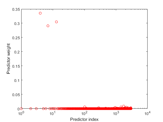
The trained GPR model assigns the largest weights to the 4th, 7th, and 13th predictors. The irrelevant predictors have weights close to zero.

Input Arguments

Tbl — Sample data

table

Sample data used to train the model, specified as a table. Each row of Tbl corresponds to one observation, and each column corresponds to one variable. Tbl contains the predictor variables, and optionally it can also contain one column for the response variable. Multicolumn variables and cell arrays other than cell arrays of character vectors are not allowed.

• If Tbl contains the response variable, and you want to use all the remaining variables as predictors, then specify the response variable using ResponseVarName.

• If Tbl contains the response variable, and you want to use only a subset of the predictors in training the model, then specify the response variable and the predictor variables using formula.

• If Tbl does not contain the response variable, then specify a response variable using y. The length of the response variable and the number of rows in Tbl must be equal.

For more information on the table data type, see table.

If your predictor data contains categorical variables, then fitrgp creates dummy variables. For details, see CategoricalPredictors.

Data Types: table

ResponseVarName — Response variable name

name of a variable in Tbl

Response variable name, specified as the name of a variable in Tbl. You must specify ResponseVarName as a character vector or string scalar. For example, if the response variable y is stored in Tbl (as Tbl.y), then specify it as "y". Otherwise, the software treats all the columns of Tbl, including y, as predictors when training the model.

Data Types: char | string

formula — Response and predictor variables to use in model training

character vector or string scalar in the form of "y~x1+x2+x3"

Response and predictor variables to use in model training, specified as a character vector or string scalar in the form of "y~x1+x2+x3". In this form, y represents the response variable; x1, x2, x3 represent the predictor variables to use in training the model.

Use a formula if you want to specify a subset of variables in Tbl as predictors to use when training the model. If you specify a formula, then any variables that do not appear in formula are not used to train the model.

The variable names in the formula must be both variable names in Tbl (Tbl.Properties.VariableNames) and valid MATLAB^® identifiers. You can verify the variable names in Tbl by using the isvarname function. If the variable names are not valid, then you can convert them by using the matlab.lang.makeValidName function.

The formula does not indicate the form of the BasisFunction.

Example: "PetalLength~PetalWidth+Species" identifies the variable PetalLength as the response variable, and PetalWidth and Species as the predictor variables.

Data Types: char | string

X — Predictor data for the GPR model

n-by-d matrix

Predictor data for the GPR model, specified as an n-by-d matrix. n is the number of observations (rows), and d is the number of predictors (columns).

The length of y and the number of rows of X must be equal.

To specify the names of the predictors in the order of their appearance in X, use the PredictorNames name-value argument.

Data Types: double

y — Response data for the GPR model

n-by-1 vector

Response data for the GPR model, specified as an n-by-1 vector. You can omit y if you provide the Tbl training data that also includes y. In that case, use ResponseVarName to identify the response variable or use formula to identify the response and predictor variables.

Data Types: double

Name-Value Arguments

Specify optional pairs of arguments as Name1=Value1,...,NameN=ValueN, where Name is the argument name and Value is the corresponding value. Name-value arguments must appear after other arguments, but the order of the pairs does not matter.

Example: FitMethod="sr",BasisFunction="linear",ActiveSetMethod="sgma",PredictMethod="fic" trains the GPR model using the subset of regressors approximation method for parameter estimation, uses a linear basis function, uses sparse greedy matrix approximation for active selection, and fully independent conditional approximation method for prediction.

Note

You cannot use any cross-validation name-value argument together with the OptimizeHyperparameters name-value argument. You can modify the cross-validation for OptimizeHyperparameters only by using the HyperparameterOptimizationOptions name-value argument.

Fitting

FitMethod — Method to estimate parameters of GPR model

"none" | "exact" | "sd" | "sr" | "fic"

Method to estimate the parameters of the GPR model, specified as one of the following.

Fit Method	Description
"none"	No estimation. Use the initial parameter values as the known parameter values.
"exact"	Exact Gaussian process regression. This value is the default if n ≤ 2000, where n is the number of observations.
"sd"	Subset of data points approximation. This value is the default if n > 2000, where n is the number of observations. "sd" is a sparse method.
"sr"	Subset of regressors approximation. "sr" is a sparse method.
"fic"	Fully independent conditional approximation. "fic" is a sparse method.

Example: FitMethod="fic"

BasisFunction — Explicit basis in GPR model

"constant" (default) | "none" | "linear" | "pureQuadratic" | function handle

Explicit basis in the GPR model, specified as "constant", "none", "linear", "pureQuadratic", or a function handle. If n is the number of observations, the basis function adds the term H*β to the model, where H is the basis matrix and β is a p-by-1 vector of basis coefficients.

Explicit Basis	Basis Matrix
"none"	Empty matrix
"constant"	$$H=1$$ H is an n-by-1 vector of 1s, where n is the number of observations.
"linear"	$$H=[1,X]$$ X is the expanded predictor data after the software creates dummy variables for the categorical variables. For details about creating dummy variables, see CategoricalPredictors.
"pureQuadratic"	$$H=\left[1,X,X_2\right],$$ where $$X_2=\left[\begin{array}{cccc}{x}_{11}^2& x_{12}^2& \cdots & x_{1d}^2\\ x_{21}^2& x_{22}^2& \cdots & x_{2d}^2\\ ⋮& ⋮& ⋮& ⋮\\ x_{n1}^2& x_{n2}^2& \cdots & x_{nd}^2\end{array}\right].$$ For this basis option, the software does not support X with categorical predictors.
Function handle	Function handle hfcn, which fitrgp calls as $$H=hfcn(X),$$ where X is an n-by-d matrix of predictors, d is the number of predictors after the software creates dummy variables for the categorical variables, and H is an n-by-p matrix of basis functions.

Example: BasisFunction="pureQuadratic"

Data Types: char | string | function_handle

Beta — Initial value of coefficients

p-by-1 vector

Initial value of the coefficients for the explicit basis, specified as a p-by-1 vector, where p is the number of columns in the basis matrix H.

The basis matrix depends on the specified basis function. For more information, see BasisFunction.

The training function uses the coefficient initial values as the known coefficient values only when FitMethod is "none".

Data Types: double

Sigma — Initial value for noise standard deviation

std(y)/sqrt(2) (default) | positive scalar value

Initial value for the noise standard deviation of the Gaussian process model, specified as a positive scalar value.

The training function parameterizes the noise standard deviation as the sum of SigmaLowerBound and exp(η), where η is an unconstrained value. Therefore, Sigma must be larger than SigmaLowerBound by a small tolerance so that the function can initialize η to a finite value. Otherwise, the function resets Sigma to a compatible value.

The tolerance is 1e-3 when ConstantSigma is false (default) and 1e-6 otherwise. If the tolerance is not small enough relative to the scale of the response variable, you can scale up the response variable so that the tolerance value can be considered small for the response variable.

Example: Sigma=2

Data Types: double

ConstantSigma — Constant value of Sigma for noise standard deviation

false or 0 (default) | true or 1

Constant value of Sigma for the noise standard deviation of the Gaussian process model, specified as a numeric or logical 0 (false) or 1 (true). When ConstantSigma is true, the training function does not optimize the value of Sigma, but instead uses the initial value throughout its computations.

Example: ConstantSigma=true

Data Types: logical

SigmaLowerBound — Lower bound on noise standard deviation

1e-2*std(y) (default) | positive scalar value

Lower bound on the noise standard deviation (Sigma), specified as a positive scalar value.

Sigma must be larger than SigmaLowerBound by a small tolerance.

Example: SigmaLowerBound=0.02

Data Types: double

CategoricalPredictors — Categorical predictors list

vector of positive integers | logical vector | character matrix | string array | cell array of character vectors | "all"

Categorical predictors list, specified as one of the values in this table.

Value	Description
Vector of positive integers	Each entry in the vector is an index value indicating that the corresponding predictor is categorical. The index values are between 1 and p, where p is the number of predictors used to train the model. If fitrgp uses a subset of input variables as predictors, then the function indexes the predictors using only the subset. The CategoricalPredictors values do not count any response variable, observation weights variable, or other variable that the function does not use.
Logical vector	A true entry means that the corresponding predictor is categorical. The length of the vector is p.
Character matrix	Each row of the matrix is the name of a predictor variable. The names must match the entries in PredictorNames. Pad the names with extra blanks so each row of the character matrix has the same length.
String array or cell array of character vectors	Each element in the array is the name of a predictor variable. The names must match the entries in PredictorNames.
"all"	All predictors are categorical.

By default, if the predictor data is in a table (Tbl), fitrgp assumes that a variable is categorical if it is a logical vector, categorical vector, character array, string array, or cell array of character vectors. If the predictor data is a matrix (X), fitrgp assumes that all predictors are continuous. To identify any other predictors as categorical predictors, specify them by using the CategoricalPredictors name-value argument.

For the identified categorical predictors, fitrgp creates dummy variables using two different schemes, depending on whether a categorical variable is unordered or ordered. For an unordered categorical variable, fitrgp creates one dummy variable for each level of the categorical variable. For an ordered categorical variable, fitrgp creates one less dummy variable than the number of categories. For details, see Automatic Creation of Dummy Variables.

Example: CategoricalPredictors="all"

Data Types: single | double | logical | char | string | cell

Standardize — Indicator to standardize data

false or 0 (default) | true or 1

Indicator to standardize data, specified as a numeric or logical 0 (false) or 1 (true).

If you set Standardize=1, then the software centers and scales each column of the predictor data by the column mean and standard deviation. The software does not standardize the data contained in the dummy variable columns generated for categorical predictors.

Example: Standardize=1

Example: Standardize=true

Data Types: logical

Regularization — Regularization standard deviation

1e-2*std(y) (default) | positive scalar value

Regularization standard deviation for the subset of regressors ("sr") and fully independent conditional ("fic") approximation methods, specified as a positive scalar value. For more information, see FitMethod.

Example: Regularization=0.2

Data Types: double

ComputationMethod — Method for computing loglikelihood and gradient

"qr" (default) | "v"

Method for computing the loglikelihood and gradient for parameter estimation, specified as "qr" or "v". This argument is valid when FitMethod is "sr" or "fic".

• "qr" — Use the QR-factorization-based approach, which provides better accuracy.

• "v" — Use the V-method-based approach, which provides faster computation.

For more information about these approaches, see Foster, et. al. [7].

Example: ComputationMethod="v"

Kernel (Covariance) Function

KernelFunction — Form of covariance function

"squaredexponential" (default) | "exponential" | "matern32" | "matern52" | "rationalquadratic" | "ardsquaredexponential" | "ardexponential" | "ardmatern32" | "ardmatern52" | "ardrationalquadratic" | function handle

Form of the covariance function, specified as one of the following.

Value	Description
"exponential"	Exponential kernel
"squaredexponential"	Squared exponential kernel
"matern32"	Matern kernel with parameter 3/2
"matern52"	Matern kernel with parameter 5/2
"rationalquadratic"	Rational quadratic kernel
"ardexponential"	Exponential kernel with a separate length scale per predictor
"ardsquaredexponential"	Squared exponential kernel with a separate length scale per predictor
"ardmatern32"	Matern kernel with parameter 3/2 and a separate length scale per predictor
"ardmatern52"	Matern kernel with parameter 5/2 and a separate length scale per predictor
"ardrationalquadratic"	Rational quadratic kernel with a separate length scale per predictor
Function handle	Function handle in the form: Kmn = kfcn(Xm,Xn,theta), where Xm is an m-by-d matrix, Xn is an n-by-d matrix, and Kmn is an m-by-n matrix of kernel products such that Kmn(i,j) is the kernel product between Xm(i,:) and Xn(j,:). d is the number of predictor variables after the software creates dummy variables for the categorical variables. For details about creating dummy variables, see CategoricalPredictors. theta is the r-by-1 unconstrained parameter vector for kfcn.

For more information on the kernel functions, see Kernel (Covariance) Function Options.

Example: KernelFunction="matern32"

Data Types: char | string | function_handle

KernelParameters — Initial values for kernel parameters

numeric vector

Initial values for the kernel parameters, specified as a numeric vector. The size of the vector and the values depend on the form of the covariance function, specified by the KernelFunction name-value argument.

KernelFunction Value	KernelParameters Value
"exponential", "squaredexponential", "matern32", or "matern52"	2-by-1 vector phi, where phi(1) contains the length scale and phi(2) contains the signal standard deviation. The default initial value of the length scale parameter is the mean of the standard deviations of the predictors. The signal standard deviation is the standard deviation of the responses divided by the square root of 2. That is, phi = [mean(std(X));std(y)/sqrt(2)].
"rationalquadratic"	3-by-1 vector phi, where phi(1) contains the length scale, phi(2) contains the scale-mixture parameter, and phi(3) contains the signal standard deviation. The default initial value of the length scale parameter is the mean of the standard deviations of the predictors. The signal standard deviation is the standard deviation of the responses divided by the square root of 2. The default initial value for the scale-mixture parameter is 1. That is, phi = [mean(std(X));1;std(y)/sqrt(2)].
"ardexponential", "ardsquaredexponential", "ardmatern32", or "ardmatern52"	(d+1)-by-1 vector phi, where phi(i) contains the length scale for predictor i, and phi(d+1) contains the signal standard deviation. d is the number of predictor variables after the software creates dummy variables for the categorical variables. For details about creating dummy variables, see CategoricalPredictors. The default initial values of the length scale parameters are the standard deviations of the predictors. The signal standard deviation is the standard deviation of the responses divided by the square root of 2. That is, phi = [std(X)';std(y)/sqrt(2)].
"ardrationalquadratic"	(d+2)-by-1 vector phi, where phi(i) contains the length scale for predictor i, phi(d+1) contains the scale-mixture parameter, and phi(d+2) contains the signal standard deviation. d is the number of predictor variables after the software creates dummy variables for the categorical variables. For details about creating dummy variables, see CategoricalPredictors. The default initial values of the length scale parameters are the standard deviations of the predictors. The signal standard deviation is the standard deviation of the responses divided by the square root of 2. The default initial value of the scale-mixture parameter is 1. That is, phi = [std(X)';1;std(y)/sqrt(2)].
Function handle	r-by-1 vector for the initial value of the unconstrained parameter vector phi for the custom kernel function kfcn. When KernelFunction is a function handle, you must supply initial values for the kernel parameters.

For more information on the kernel functions, see Kernel (Covariance) Function Options.

Example: KernelParameters=phi

Data Types: double | single

DistanceMethod — Method for computing inter-point distances

"fast" (default) | "accurate"

Method for computing inter-point distances to evaluate built-in kernel functions, specified as "fast" or "accurate". When you specify "fast", the training function computes $${\left(x-y\right)}^2$$ as $$x^2+y^2-2*x*y$$. When you specify "accurate", the training function computes $${\left(x-y\right)}^2$$.

Example: DistanceMethod="accurate"

Active Set Selection

ActiveSet — Observations in the active set

[] (default) | m-by-1 vector of integers ranging from 1 to n (m ≤ n) | logical vector of length n

Observations in the active set, specified as an m-by-1 vector of integers ranging from 1 to n (m ≤ n) or a logical vector of length n with at least one true element. n is the total number of observations in the training data.

fitrgp uses the observations indicated by ActiveSet to train the GPR model. The active set cannot have duplicate elements.

If you supply ActiveSet, then:

• fitrgp does not use ActiveSetSize and ActiveSetMethod.

• You cannot perform cross-validation on this model.

Data Types: double | logical

ActiveSetSize — Size of active set

integer m (1 ≤ m ≤ n)

Size of the active set, specified as an integer m, 1 ≤ m ≤ n, where n is the number of observations. This argument is valid when FitMethod is "sd", "sr", or "fic".

The default value is min(1000,n) when FitMethod is "sr" or "fic", and min(2000,n) otherwise.

Example: ActiveSetSize=100

Data Types: double

ActiveSetMethod — Active set selection method

"random" (default) | "sgma" | "entropy" | "likelihood"

Active set selection method, specified as one of the following values.

Value	Description
"random"	Random selection
"sgma"	Sparse greedy matrix approximation
"entropy"	Differential entropy-based selection
"likelihood"	Subset of regressors loglikelihood-based selection

All active set selection methods (except "random") require the storage of an n-by-m matrix, where m is the size of the active set and n is the number of observations.

Example: ActiveSetMethod="entropy"

RandomSearchSetSize — Random search set size

59 (default) | integer value

Random search set size per greedy inclusion for active set selection, specified as an integer value.

Example: RandomSearchSetSize=30

Data Types: double

ToleranceActiveSet — Relative tolerance for terminating active set selection

1e-06 (default) | positive scalar

Relative tolerance for terminating active set selection, specified as a positive scalar.

Example: ToleranceActiveset=0.0002

Data Types: double

NumActiveSetRepeats — Number of repetitions

3 (default) | integer value

Number of repetitions for interleaved active set selection and parameter estimation when ActiveSetMethod is not "random", specified as an integer value.

Example: NumActiveSetRepeats=5

Data Types: double

Prediction

PredictMethod — Method used to make predictions

"exact" | "bcd" | "sd" | "sr" | "fic"

Method used to make predictions from a Gaussian process model given the parameters, specified as one of the following values.

Value	Description
"exact"	Exact Gaussian process regression method. This value is the default if n ≤ 10,000.
"bcd"	Block coordinate descent (BCD). This value is the default if n > 10,000.
"sd"	Subset of data points approximation
"sr"	Subset of regressors approximation
"fic"	Fully independent conditional approximation

Example: PredictMethod="bcd"

BlockSizeBCD — Block size for BCD method

minimum of 1000 or n (default) | integer in the range 1 to n

Block size for the block coordinate descent method ("bcd"), specified as an integer in the range 1 to n, where n is the number of observations.

Example: BlockSizeBCD=1500

Data Types: double

NumGreedyBCD — Number of greedy selections for BCD method

minimum of 100 and BlockSizeBCD (default) | integer value in the range 1 to BlockSizeBCD

Number of greedy selections for the block coordinate descent method ("bcd"), specified as an integer in the range 1 to BlockSizeBCD.

Example: NumGreedyBCD=150

Data Types: double

ToleranceBCD — Relative tolerance on gradient norm

1e-3 (default) | positive scalar

Relative tolerance on the gradient norm for terminating the block coordinate descent method ("bcd") iterations, specified as a positive scalar.

Example: ToleranceBCD=0.002

Data Types: double

StepToleranceBCD — Absolute tolerance on step size

1e-3 (default) | positive scalar

Absolute tolerance on the step size for terminating the block coordinate descent method ("bcd") iterations, specified as a positive scalar.

Example: StepToleranceBCD=0.002

Data Types: double

IterationLimitBCD — Maximum number of BCD iterations

1000000 (default) | positive integer

Maximum number of block coordinate descent method ("bcd") iterations, specified as a positive integer.

Example: IterationLimitBCD=10000

Data Types: double

Optimization

Optimizer — Optimizer to use for parameter estimation

"quasinewton" (default) | "lbfgs" | "fminsearch" | "fminunc" | "fmincon"

Optimizer to use for parameter estimation, specified as one of the values in this table.

Value	Description
"quasinewton"	Dense, symmetric rank-1-based, quasi-Newton approximation to the Hessian
"lbfgs"	LBFGS-based quasi-Newton approximation to the Hessian
"fminsearch"	Unconstrained nonlinear optimization using the simplex search method of Lagarias et al. [5]
"fminunc"	Unconstrained nonlinear optimization (requires an Optimization Toolbox™ license)
"fmincon"	Constrained nonlinear optimization (requires an Optimization Toolbox license)

For more information on the optimizers, see Algorithms.

Example: Optimizer="fmincon"

OptimizerOptions — Options for optimizer

structure | object

Options for the optimizer set by the Optimizer name-value argument, specified as a structure or object created by optimset, statset("fitrgp"), or optimoptions.

Optimizer	Function for Creating Optimizer Options
"fminsearch"	optimset (structure)
"quasinewton" or "lbfgs"	statset("fitrgp") (structure)
"fminunc" or "fmincon"	optimoptions (object)

The default options depend on the specified optimizer.

Example: OptimizerOptions=opt

InitialStepSize — Initial step size

[] (default) | real positive scalar | "auto"

Initial step size, specified as a real positive scalar or "auto".

InitialStepSize is the approximate maximum absolute value of the first optimization step when the optimizer is "quasinewton" or "lbfgs". The initial step size can determine the initial Hessian approximation during optimization.

By default, the training function does not use the initial step size to determine the initial Hessian approximation. To use the initial step size, set a value for the InitialStepSize name-value argument, or specify InitialStepSize="auto" to have the software determine a value automatically. For more information on "auto", see Algorithms.

Example: InitialStepSize="auto"

Cross-Validation

CrossVal — Flag to train cross-validated model

"off" (default) | "on"

Flag to train a cross-validated model, specified as "on" or "off".

If you specify "on", then the software trains a cross-validated model with 10 folds.

You can override this cross-validation setting using the CVPartition, Holdout, KFold, or Leaveout name-value argument. You can use only one cross-validation name-value argument at a time to create a cross-validated model.

Alternatively, cross-validate later by passing Mdl to crossval.

Example: Crossval="on"

Data Types: char | string

CVPartition — Cross-validation partition

[] (default) | cvpartition object

Cross-validation partition, specified as a cvpartition object that specifies the type of cross-validation and the indexing for the training and validation sets.

To create a cross-validated model, you can specify only one of these four name-value arguments: CVPartition, Holdout, KFold, or Leaveout.

Example: Suppose you create a random partition for 5-fold cross-validation on 500 observations by using cvp = cvpartition(500,KFold=5). Then, you can specify the cross-validation partition by setting CVPartition=cvp.

Holdout — Fraction of data for holdout validation

scalar value in the range (0,1)

Fraction of the data used for holdout validation, specified as a scalar value in the range (0,1). If you specify Holdout=p, then the software completes these steps:

1. Randomly select and reserve p*100% of the data as validation data, and train the model using the rest of the data.

2. Store the compact trained model in the Trained property of the cross-validated model.

To create a cross-validated model, you can specify only one of these four name-value arguments: CVPartition, Holdout, KFold, or Leaveout.

Example: Holdout=0.1

Data Types: double | single

KFold — Number of folds

10 (default) | positive integer value greater than 1

Number of folds to use in the cross-validated model, specified as a positive integer value greater than 1. If you specify KFold=k, then the software completes these steps:

1. Randomly partition the data into k sets.

2. For each set, reserve the set as validation data, and train the model using the other k – 1 sets.

3. Store the k compact trained models in a k-by-1 cell vector in the Trained property of the cross-validated model.

To create a cross-validated model, you can specify only one of these four name-value arguments: CVPartition, Holdout, KFold, or Leaveout.

Example: KFold=5

Data Types: single | double

Leaveout — Leave-one-out cross-validation flag

"off" (default) | "on"

Leave-one-out cross-validation flag, specified as "on" or "off". If you specify Leaveout="on", then for each of the n observations (where n is the number of observations, excluding missing observations, specified in the NumObservations property of the model), the software completes these steps:

1. Reserve the one observation as validation data, and train the model using the other n – 1 observations.

2. Store the n compact trained models in an n-by-1 cell vector in the Trained property of the cross-validated model.

To create a cross-validated model, you can specify only one of these four name-value arguments: CVPartition, Holdout, KFold, or Leaveout.

Example: Leaveout="on"

Data Types: char | string

Hyperparameter Optimization

OptimizeHyperparameters — Parameters to optimize

"none" (default) | "auto" | "all" | string array or cell array of eligible parameter names | vector of optimizableVariable objects

Parameters to optimize, specified as one of the following:

• "none" — Do not optimize.

• "auto" — Use ["Sigma","Standardize"].

• "all" — Optimize all eligible parameters, equivalent to ["BasisFunction","KernelFunction","KernelScale","Sigma","Standardize"].

• String array or cell array of eligible parameter names.

• Vector of optimizableVariable objects, typically the output of hyperparameters.

The optimization attempts to minimize the cross-validation loss (error) for fitrgp by varying the parameters. To control the cross-validation type and other aspects of the optimization, use the HyperparameterOptimizationOptions name-value argument. When you use HyperparameterOptimizationOptions, you can use the (compact) model size instead of the cross-validation loss as the optimization objective by setting the ConstraintType and ConstraintBounds options.

Note

The values of OptimizeHyperparameters override any values you specify using other name-value arguments. For example, setting OptimizeHyperparameters to "auto" causes fitrgp to optimize hyperparameters corresponding to the "auto" option and to ignore any specified values for the hyperparameters.

The eligible parameters for fitrgp are:

• BasisFunction — fitrgp searches among "constant", "none", "linear", and "pureQuadratic".

• KernelFunction — fitrgp searches among "ardexponential", "ardmatern32", "ardmatern52", "ardrationalquadratic", "ardsquaredexponential", "exponential", "matern32", "matern52", "rationalquadratic", and "squaredexponential".

• KernelScale — fitrgp uses the KernelParameters argument to specify the value of the kernel scale parameter, which is held constant during fitting. In this case, all input dimensions are constrained to have the same KernelScale value. fitrgp searches among positive values log-scaled in the range [1e-3,1e3].

  KernelScale cannot be optimized for any of the ARD kernels.

• Sigma — fitrgp searches among positive values log-scaled in the range [1e-4,max(1e-3,10*ResponseStd)], where

  ResponseStd = std(y).

  Internally, fitrgp sets the ConstantSigma name-value argument to true so the value of Sigma is constant during the fitting.

• Standardize — fitrgp searches among true and false.

Set nondefault parameters by passing a vector of optimizableVariable objects that have nondefault values. For example,

load fisheriris
params = hyperparameters("fitrgp",meas,species);
params(1).Range = [1e-4,1e6];

Pass params as the value of OptimizeHyperparameters.

By default, the iterative display appears at the command line, and plots appear according to the number of hyperparameters in the optimization. For the optimization and plots, the objective function is log(1 + cross-validation loss). To control the iterative display, set the Verbose option of the HyperparameterOptimizationOptions name-value argument. To control the plots, set the ShowPlots option of the HyperparameterOptimizationOptions name-value argument.

For an example, see Optimize GPR Model.

Example: OptimizeHyperparameters="auto"

HyperparameterOptimizationOptions — Options for optimization

HyperparameterOptimizationOptions object | structure

Options for optimization, specified as a HyperparameterOptimizationOptions object or a structure. This argument modifies the effect of the OptimizeHyperparameters name-value argument. If you specify HyperparameterOptimizationOptions, you must also specify OptimizeHyperparameters. All the options are optional. However, you must set ConstraintBounds and ConstraintType to return AggregateOptimizationResults. The options that you can set in a structure are the same as those in the HyperparameterOptimizationOptions object.

Option	Values	Default
Optimizer	"bayesopt" — Use Bayesian optimization. Internally, this setting calls bayesopt. "gridsearch" — Use grid search with NumGridDivisions values per dimension. "gridsearch" searches in a random order, using uniform sampling without replacement from the grid. After optimization, you can get a table in grid order by using the sortrows function. "randomsearch" — Search at random among MaxObjectiveEvaluations points.	"bayesopt"
ConstraintBounds	Constraint bounds for N optimization problems, specified as an N-by-2 numeric matrix or []. The columns of ConstraintBounds contain the lower and upper bound values of the optimization problems. If you specify ConstraintBounds as a numeric vector, the software assigns the values to the second column of ConstraintBounds, and zeros to the first column. If you specify ConstraintBounds, you must also specify ConstraintType.	[]
ConstraintTarget	Constraint target for the optimization problems, specified as "matlab" or "coder". If ConstraintBounds and ConstraintType are [] and you set ConstraintTarget, then the software sets ConstraintTarget to []. The values of ConstraintTarget and ConstraintType determine the objective and constraint functions. For more information, see HyperparameterOptimizationOptions.	If you specify ConstraintBounds and ConstraintType, then the default value is "matlab". Otherwise, the default value is [].
ConstraintType	Constraint type for the optimization problems, specified as "size" or "loss". If you specify ConstraintType, you must also specify ConstraintBounds. The values of ConstraintTarget and ConstraintType determine the objective and constraint functions. For more information, see HyperparameterOptimizationOptions.	[]
AcquisitionFunctionName	Type of acquisition function: "expected-improvement-per-second-plus" "expected-improvement" "expected-improvement-plus" "expected-improvement-per-second" "lower-confidence-bound" "probability-of-improvement" Acquisition functions whose names include per-second do not yield reproducible results, because the optimization depends on the run time of the objective function. Acquisition functions whose names include plus modify their behavior when they overexploit an area. For more details, see Acquisition Function Types.	"expected-improvement-per-second-plus"
LossFun	Type of validation loss to optimize, specified as "auto" or "mse". In the case of fitrgp, the two options are equivalent, and the software uses the mean squared error.	"auto"
MaxObjectiveEvaluations	Maximum number of objective function evaluations. If you specify multiple optimization problems using ConstraintBounds, the value of MaxObjectiveEvaluations applies to each optimization problem individually.	30 for "bayesopt" and "randomsearch", and the entire grid for "gridsearch"
MaxTime	Time limit for the optimization, specified as a nonnegative real scalar. The time limit is in seconds, as measured by tic and toc. The software performs at least one optimization iteration, regardless of the value of MaxTime. The run time can exceed MaxTime because MaxTime does not interrupt function evaluations. If you specify multiple optimization problems using ConstraintBounds, the time limit applies to each optimization problem individually.	Inf
NumGridDivisions	For Optimizer="gridsearch", the number of values in each dimension. The value can be a vector of positive integers giving the number of values for each dimension, or a scalar that applies to all dimensions. The software ignores this option for categorical variables.	10
ShowPlots	Logical value indicating whether to show plots of the optimization progress. If this option is true, the software plots the best observed objective function value against the iteration number. If you use Bayesian optimization (Optimizer="bayesopt"), the software also plots the best estimated objective function value. The best observed objective function values and best estimated objective function values correspond to the values in the BestSoFar (observed) and BestSoFar (estim.) columns of the iterative display, respectively. You can find these values in the properties ObjectiveMinimumTrace and EstimatedObjectiveMinimumTrace of the SupervisedLearningBayesianOptimization object. If the problem includes one or two optimization parameters for Bayesian optimization, then ShowPlots also plots a model of the objective function against the parameters.	true
SaveIntermediateResults	Logical value indicating whether to save the optimization results. If this option is true, the software overwrites a workspace variable named SupervisedLearningBayesoptResults at each iteration. The variable is a SupervisedLearningBayesianOptimization object. If you specify multiple optimization problems using ConstraintBounds, the workspace variable is an AggregateBayesianOptimization object named AggregateBayesoptResults.	false
Verbose	Display level at the command line: 0 — No iterative display 1 — Iterative display 2 — Iterative display with additional information For details, see the bayesopt Verbose name-value argument and the example Optimize Classifier Fit Using Bayesian Optimization.	1
UseParallel	Logical value indicating whether to run the Bayesian optimization in parallel, which requires Parallel Computing Toolbox™. Due to the nonreproducibility of parallel timing, parallel Bayesian optimization does not necessarily yield reproducible results. For details, see Parallel Bayesian Optimization.	false
Repartition	Logical value indicating whether to repartition the cross-validation at every iteration. If this option is false, the optimizer uses a single partition for the optimization. A value of true usually gives the most robust results because this setting takes partitioning noise into account. However, for optimal results, true requires at least twice as many function evaluations.	false
Specify only one of the following three options.
CVPartition	cvpartition object created by cvpartition	KFold=5 if you do not specify a cross-validation option
Holdout	Scalar in the range (0,1) representing the holdout fraction
KFold	Integer greater than 1

Example: HyperparameterOptimizationOptions=struct(UseParallel=true)

Other

PredictorNames — Predictor variable names

string array of unique names | cell array of unique character vectors

Predictor variable names, specified as a string array of unique names or cell array of unique character vectors. The functionality of PredictorNames depends on the way you supply the training data.

• If you supply X and Y, then you can use PredictorNames to assign names to the predictor variables in X.

  • The order of the names in PredictorNames must correspond to the predictor order in X. Assuming that X has the default orientation, with observations in rows and predictors in columns, PredictorNames{1} is the name of X(:,1), PredictorNames{2} is the name of X(:,2), and so on. Also, size(X,2) and numel(PredictorNames) must be equal.

  • By default, PredictorNames is {'x1','x2',...}.

• If you supply Tbl, then you can use PredictorNames to choose which predictor variables to use in training. That is, fitrgp uses only the variables in PredictorNames as predictors during training.

  • PredictorNames must be a subset of Tbl.Properties.VariableNames and cannot include the name of any response variable.

  • By default, PredictorNames contains the names of all predictor variables.

  • A good practice is to specify the predictors for training using either PredictorNames or formula, but not both.

Example: PredictorNames=["SepalLength","SepalWidth","PetalLength","PetalWidth"]

Data Types: string | cell

ResponseName — Response variable name

"Y" (default) | character vector | string scalar

Response variable name, specified as a character vector or string scalar.

• If you supply Y, then you can use ResponseName to specify a name for the response variable.

• If you supply ResponseVarName or formula, then you cannot use ResponseName.

Example: ResponseName="response"

Data Types: char | string

Verbose — Verbosity level

0 (default) | 1

Verbosity level, specified as 0 or 1.

• 0 — The training function suppresses diagnostic messages related to active set selection and block coordinate descent, but displays the messages related to parameter estimation, depending on the value of Display in OptimizerOptions.

• 1 — The training function displays the iterative diagnostic messages related to parameter estimation, active set selection, and block coordinate descent.

Example: Verbose=1

CacheSize — Cache size in megabytes

1000 (default) | positive scalar

Cache size in megabytes (MB), specified as a positive scalar. Cache size is the extra memory available in addition to the memory required for fitting and active set selection. The training function uses CacheSize to:

• Decide whether inter-point distances are cached when estimating parameters.

• Decide how matrix vector products are computed for the block coordinate descent method and for making predictions.

Example: CacheSize=2000

Data Types: double

Output Arguments

Mdl — Trained Gaussian process regression model

RegressionGP object | RegressionPartitionedGP object | cell array of model objects

Trained Gaussian process regression model, returned as a RegressionGP object, a RegressionPartitionedGP object, or a cell array of model objects.

• If you set any of the name-value arguments CrossVal, CVPartition, Holdout, KFold, or Leaveout, then Mdl is a RegressionPartitionedGP object.

• If you specify OptimizeHyperparameters and set the ConstraintType and ConstraintBounds options of HyperparameterOptimizationOptions, then Mdl is an N-by-1 cell array of model objects, where N is equal to the number of rows in ConstraintBounds. If none of the optimization problems yields a feasible model, then each cell array value is [].

• Otherwise, Mdl is a RegressionGP model object.

To reference properties of a model object, use dot notation.

AggregateOptimizationResults — Aggregate optimization results

AggregateBayesianOptimization object

Aggregate optimization results for multiple optimization problems, returned as an AggregateBayesianOptimization object. To return AggregateOptimizationResults, you must specify OptimizeHyperparameters and HyperparameterOptimizationOptions. You must also specify the ConstraintType and ConstraintBounds options of HyperparameterOptimizationOptions. For an example that shows how to produce this output, see Hyperparameter Optimization with Multiple Constraint Bounds.

More About

Active Set Selection and Parameter Estimation

For subset of data, subset of regressors, or fully independent conditional approximation fitting methods (FitMethod equal to "sd", "sr", or "fic"), if you do not provide the active set (or inducing input set), fitrgp selects the active set and computes the parameter estimates in a series of iterations.

In the first iteration, the software uses the initial parameter values in vector η₀ = [β₀,σ₀,θ₀] to select an active set A₁. The software maximizes the GPR marginal loglikelihood or its approximation using η₀ as the initial values and A₁ to compute the new parameter estimates η₁. Next, the software computes the new loglikelihood L₁ using η₁ and A₁.

In the second iteration, the software selects the active set A₂ using the parameter values in η₁. Then, using η₁ as the initial values and A₂, the software maximizes the GPR marginal loglikelihood or its approximation and estimates the new parameter values η₂. Then, using η₂ and A₂, the software computes the new loglikelihood value L₂.

The following table summarizes the iterations and the computations at each iteration.

Iteration Number	Active Set	Parameter Vector	Loglikelihood
1	A1	η1	L1
2	A2	η2	L2
3	A3	η3	L3
…	…	…	…

The software iterates similarly for a specified number of repetitions. You can specify the number of replications for active set selection using the NumActiveSetRepeats name-value argument.

Tips

• fitrgp accepts any combination of fitting, prediction, and active set selection methods. In some cases it might not be possible to compute the standard deviations of the predicted responses, hence the prediction intervals. See predict. And in some cases, using the exact method might be expensive due to the size of the training data.

• The PredictorNames property stores one element for each of the original predictor variable names. For example, if there are three predictors, one of which is a categorical variable with three levels, PredictorNames is a 1-by-3 cell array of character vectors.

• The ExpandedPredictorNames property stores one element for each of the predictor variables, including the dummy variables. For example, if there are three predictors, one of which is a categorical variable with three levels, then ExpandedPredictorNames is a 1-by-5 cell array of character vectors.

• Similarly, the Beta property stores one beta coefficient for each predictor, including the dummy variables.

• The X property stores the training data as originally input. It does not include the dummy variables.

• The default approach to initializing the Hessian approximation in fitrgp can be slow when you have a GPR model with many kernel parameters, such as when using an ARD kernel with many predictors. In this case, consider specifying "auto" or a value for the initial step size.

  You can set Verbose=1 for display of iterative diagnostic messages, and begin training a GPR model using an LBFGS or quasi-Newton optimizer with the default fitrgp optimization. If the iterative diagnostic messages are not displayed after a few seconds, it is possible that initialization of the Hessian approximation is taking too long. In this case, consider restarting training and using the initial step size to speed up optimization.

• After training a model, you can generate C/C++ code that predicts responses for new data. Generating C/C++ code requires MATLAB Coder™. For details, see Introduction to Code Generation for Statistics and Machine Learning Functions..

Algorithms

• Fitting a GPR model involves estimating the following model parameters from the data:

  • Covariance function $$k\left(x_i,x_j|\theta \right)$$ parameterized in terms of kernel parameters in vector $$\theta$$ (see Kernel (Covariance) Function Options)

  • Noise variance $${\sigma }^2$$

  • Coefficient vector of fixed-basis functions $$\beta$$

  The value of the KernelParameters name-value argument is a vector that consists of initial values for the signal standard deviation $${\sigma }_f$$ and the characteristic length scales $${\sigma }_l$$. The software uses these values to determine the kernel parameters. Similarly, the Sigma name-value argument contains the initial value for the noise standard deviation $$\sigma$$.

• During optimization, the software creates a vector of unconstrained initial parameter values $${\eta }_0$$ by using the initial values for the noise standard deviation and the kernel parameters.

• The software analytically determines the explicit basis coefficients $$\beta$$, specified by the Beta name-value argument, from estimated values of $$\theta$$ and $${\sigma }^2$$. Therefore, $$\beta$$ does not appear in the $${\eta }_0$$ vector when the software initializes numerical optimization.

  Note

  If you do not specify the estimation of parameters for the GPR model, the software uses the value of the Beta name-value argument and other initial parameter values as the known GPR parameter values (see Beta). In all other cases, the value of Beta is optimized analytically from the objective function.

• The quasi-Newton optimizer uses a trust-region method with a dense, symmetric rank-1-based (SR1), quasi-Newton approximation to the Hessian. The LBFGS optimizer uses a standard line-search method with a limited-memory Broyden-Fletcher-Goldfarb-Shanno (LBFGS) quasi-Newton approximation to the Hessian. See Nocedal and Wright [6].

• If you set the InitialStepSize name-value argument to "auto" the software determines the initial step size $${\Vert s_0\Vert }_{\infty }$$ by using $${\Vert s_0\Vert }_{\infty }=0.5{\Vert {\eta }_0\Vert }_{\infty }+0.1$$.

  $$s_0$$ is the initial step vector, and $${\eta }_0$$ is the vector of unconstrained initial parameter values.

• During optimization, the software uses the initial step size $${\Vert s_0\Vert }_{\infty }$$ as follows:

  If you specify Optimizer="quasinewton" with the initial step size, then the initial Hessian approximation is $$\frac{{\Vert g_0\Vert }_{\infty }}{{\Vert s_0\Vert }_{\infty }}I$$.

  If you specify Optimizer="lbfgs" with the initial step size, then the initial inverse-Hessian approximation is $$\frac{{\Vert s_0\Vert }_{\infty }}{{\Vert g_0\Vert }_{\infty }}I$$.

  $$g_0$$ is the initial gradient vector, and $$I$$ is the identity matrix.

References

[1] Nash, W.J., T. L. Sellers, S. R. Talbot, A. J. Cawthorn, and W. B. Ford. "The Population Biology of Abalone (Haliotis species) in Tasmania. I. Blacklip Abalone (H. rubra) from the North Coast and Islands of Bass Strait." Sea Fisheries Division, Technical Report No. 48, 1994.

[2] Waugh, S. "Extending and Benchmarking Cascade-Correlation: Extensions to the Cascade-Correlation Architecture and Benchmarking of Feed-forward Supervised Artificial Neural Networks." University of Tasmania Department of Computer Science thesis, 1995.

[3] Lichman, M. UCI Machine Learning Repository, Irvine, CA: University of California, School of Information and Computer Science, 2013. http://archive.ics.uci.edu/ml.

[4] Rasmussen, C. E. and C. K. I. Williams. Gaussian Processes for Machine Learning. MIT Press. Cambridge, Massachusetts, 2006.

[5] Lagarias, J. C., J. A. Reeds, M. H. Wright, and P. E. Wright. "Convergence Properties of the Nelder-Mead Simplex Method in Low Dimensions." SIAM Journal of Optimization. Vol. 9, Number 1, 1998, pp. 112–147.

[6] Nocedal, J. and S. J. Wright. Numerical Optimization, Second Edition. Springer Series in Operations Research, Springer Verlag, 2006.

Extended Capabilities

Automatic Parallel Support

Accelerate code by automatically running computation in parallel using Parallel Computing Toolbox™.

To perform parallel hyperparameter optimization, use the UseParallel=true option in the HyperparameterOptimizationOptions name-value argument in the call to the fitrgp function.

For more information on parallel hyperparameter optimization, see Parallel Bayesian Optimization.

For general information about parallel computing, see Run MATLAB Functions with Automatic Parallel Support (Parallel Computing Toolbox).

GPU Arrays

Accelerate code by running on a graphics processing unit (GPU) using Parallel Computing Toolbox™. (since R2026a)

• fitrgp fits the model on a GPU if at least one of the following applies:

  • The input argument X is a gpuArray object.

  • The input argument Y is a gpuArray object.

  • The input argument Tbl contains gpuArray predictor or response variables.

For more information, see Run MATLAB Functions on a GPU (Parallel Computing Toolbox).

Version History

Introduced in R2015b

R2026a: Specify gpuArray inputs (requires Parallel Computing Toolbox)

fitrgp supports GPU array input arguments.

R2025a: Compute serially when parallel hyperparameter optimization is not available

fitrgp defaults to serial hyperparameter optimization when HyperparameterOptimizationOptions includes UseParallel=true and the software cannot open a parallel pool.

In previous releases, the software issues an error under these circumstances.

R2023b: "auto" option of OptimizeHyperparameters includes Standardize

Starting in R2023b, when you specify "auto" as the OptimizeHyperparameters value, fitrgp includes Standardize as an optimizable hyperparameter.

R2023b: KernelScale hyperparameter search range does not depend on predictor data during optimization of GPR models

Starting in R2023b, fitrgp optimizes the kernel scale parameter for Gaussian process regression (GPR) models by using the default search range [1e-3,1e3]. That is, when you specify to optimize the GPR hyperparameter KernelScale by using the OptimizeHyperparameters name-value argument, the function searches among positive values log-scaled in the range [1e-3,1e3].

In previous releases, the default search range for the KernelScale hyperparameter was [1e-3*MaxPredictorRange,MaxPredictorRange], where MaxPredictorRange = max(max(X) - min(X)).

R2022b: A cross-validated Gaussian process regression model is a RegressionPartitionedGP object

Starting in R2022b, a cross-validated Gaussian process regression (GPR) model is a RegressionPartitionedGP object. In previous releases, a cross-validated GPR model was a RegressionPartitionedModel object.

You can create a RegressionPartitionedGP object in two ways:

• Create a cross-validated model from a GPR model object RegressionGP by using the crossval object function.

• Create a cross-validated model by using the fitrgp function and specifying one of the name-value arguments CrossVal, CVPartition, Holdout, KFold, or Leaveout.

Regardless of whether you train a full or cross-validated GPR model first, you cannot specify an ActiveSet value in the call to fitrgp.