Weibull Distribution

Overview

The Weibull distribution is a two-parameter family of curves. This distribution is named for Waloddi Weibull, who offered it as an appropriate analytical tool for modeling the breaking strength of materials. Current usage also includes reliability and lifetime modeling. The Weibull distribution is more flexible than the exponential distribution for these purposes, because the exponential distribution has a constant hazard function.

Statistics and Machine Learning Toolbox™ offers several ways to work with the Weibull distribution.

• Create a probability distribution object WeibullDistribution by fitting a probability distribution to sample data (fitdist) or by specifying parameter values (makedist). Then, use object functions to evaluate the distribution, generate random numbers, and so on.

• Work with the Weibull distribution interactively by using the Distribution Fitter app. You can export an object from the app and use the object functions.

• Use distribution-specific functions (wblcdf, wblpdf, wblinv, wbllike, wblstat, wblfit, wblrnd, wblplot) with specified distribution parameters. The distribution-specific functions can accept parameters of multiple Weibull distributions.

• Use generic distribution functions (cdf, icdf, pdf, random) with a specified distribution name ('Weibull') and parameters.

Parameters

Statistics and Machine Learning Toolbox functions use a two-parameter Weibull distribution with these parameters.

Parameter	Description	Support
a	Scale	a > 0
b	Shape	b > 0

The standard Weibull distribution has unit scale.

The Weibull distribution can take a third parameter. The three-parameter Weibull distribution adds a location parameter that is zero in the two-parameter case. If X has a two-parameter Weibull distribution, then Y = X + c has a three-parameter Weibull distribution with the added location parameter c. For more details, see Three-Parameter Weibull Distribution.

Parameter Estimation

The likelihood function is the probability density function (pdf) viewed as a function of the parameters. The maximum likelihood estimates (MLEs) are the parameter estimates that maximize the likelihood function for fixed values of x. The maximum likelihood estimators of a and b for the Weibull distribution are the solution of the simultaneous equations

$$\begin{array}{l}\widehat{a}={\left[\left(\frac{1}{n}\right){\displaystyle \sum _{i=1}^n{x}_i^{\widehat{b}}}\right]}^{\frac{1}{\widehat{b}}}\\ \widehat{b}=\frac{n}{\left(\frac{1}{\widehat{a}}\right){\displaystyle \sum _{i=1}^n{x}_i^{\widehat{b}}\log x_i}-{\displaystyle \sum _{i=1}^n\log x_i}}.\end{array}$$

â and $$\widehat{b}$$ are unbiased estimators of the parameters a and b.

To fit the Weibull distribution to data and find parameter estimates, use wblfit, fitdist, or mle. Unlike wblfit and mle, which return parameter estimates, fitdist returns the fitted probability distribution object WeibullDistribution. The object properties a and b store the parameter estimates.

For an example, see Fit Weibull Distribution to Data and Estimate Parameters.

Probability Density Function

The pdf of the Weibull distribution is

$$f\left(x|a,b\right)=\{\begin{array}{ll}\frac{b}{a}{\left(\frac{x}{a}\right)}^{b-1}{e}^{-{\left(x/a\right)}^b}\hfill & \text{if }x\ge 0,\hfill \\ 0\hfill & \text{if }x<0.\hfill \end{array}$$

For an example, see Compute Weibull Distribution pdf.

Cumulative Distribution Function

The cumulative distribution function (cdf) of the Weibull distribution is

$$p=F\left(x|a,b\right)={\displaystyle {\int }_0^{x}b{a}^{-b}{t}^{b-1}{e}^{-{\left(\frac{t}{a}\right)}^b}dt}=1-e^{-{\left(\frac{x}{a}\right)}^b}.$$

The result p is the probability that a single observation from a Weibull distribution with parameters a and b falls in the interval [0 x].

For an example, see Compute Weibull Distribution cdf.

Inverse Cumulative Distribution Function

The inverse cdf of the Weibull distribution is

$$x=F^{-1}(p|a,b)=-a{\left[\ln \left(1-p\right)\right]}^{1/b}.$$

The result x is the value where an observation from a Weibull distribution with parameters a and b falls in the range [0 x] with probability p.

Hazard Function

The hazard function (instantaneous failure rate) is the ratio of the pdf and the complement of the cdf. If f(t) and F(t) are the pdf and cdf of a distribution, then the hazard rate is $$h\left(t\right)=\frac{f\left(t\right)}{1-F\left(t\right)}$$. Substituting the pdf and cdf of the exponential distribution for f(t) and F(t) above yields the function $$\frac{b}{a^b}{x}^{b-1}$$.

For an example, see Compare Exponential and Weibull Distribution Hazard Functions.

Examples

Fit Weibull Distribution to Data and Estimate Parameters

Simulate the tensile strength data of a thin filament using the Weibull distribution with the scale parameter value 0.5 and the shape parameter value 2.

rng('default');                  % For reproducibility
strength = wblrnd(0.5,2,100,1);  % Simulated strengths

Compute the MLEs and confidence intervals for the Weibull distribution parameters.

[param,ci] = wblfit(strength)

param = 1×2

    0.4768    1.9622

ci = 2×2

    0.4291    1.6821
    0.5298    2.2890

The estimated scale parameter is 0.4768, with the 95% confidence interval (0.4291,0.5298).

The estimated shape parameter is 1.9622, with the 95% confidence interval (1.6821,2.2890).

The default confidence interval for each parameter contains the true value.

Compute Weibull Distribution pdf

Compute and plot the pdf of the Weibull distribution for various values of the scale (A) and shape (B) parameters.

x = linspace(0,30);
plot(x,wblpdf(x,10,1),'DisplayName','A=10, B=1')
hold on
plot(x,wblpdf(x,10,2),'DisplayName','A=10, B=2')
plot(x,wblpdf(x,10,4),'DisplayName','A=10, B=4')
plot(x,wblpdf(x,10,0.5),'DisplayName','A=10, B=0.5')
plot(x,wblpdf(x,10,0.25),'DisplayName','A=10, B=0.25')
plot(x,wblpdf(x,5,1),'DisplayName','A=5, B=1')
hold off
legend('show')
xlabel('x')
ylabel('pdf')

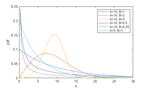
The value B=1 leads to the exponential distribution. Values of B<1 have a density that approaches infinity as x approaches 0. Values of B>1 have a density that approaches 0 as x approaches 1.

Compute Weibull Distribution cdf

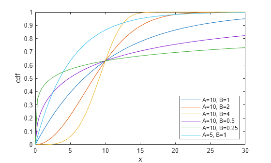
Compute and plot the cdf of the Weibull distribution for various values of the scale (A) and shape (B) parameters.

x = linspace(0,30);
plot(x,wblcdf(x,10,1),'DisplayName','A=10, B=1')
hold on
plot(x,wblcdf(x,10,2),'DisplayName','A=10, B=2')
plot(x,wblcdf(x,10,4),'DisplayName','A=10, B=4')
plot(x,wblcdf(x,10,0.5),'DisplayName','A=10, B=0.5')
plot(x,wblcdf(x,10,0.25),'DisplayName','A=10, B=0.25')
plot(x,wblcdf(x,5,1),'DisplayName','A=5, B=1')
hold off
legend('Location','southeast')
xlabel('x')
ylabel('cdf')

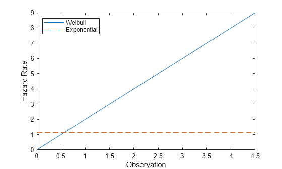
Compare Exponential and Weibull Distribution Hazard Functions

The exponential distribution has a constant hazard function, which is not generally the case for the Weibull distribution. In this example, the Weibull hazard rate increases with age (a reasonable assumption).

Compute the hazard function for the Weibull distribution with the scale parameter value 1 and the shape parameter value 2.

t = 0:0.1:4.5;
h1 = wblpdf(t,1,2)./(1-wblcdf(t,1,2));

Compute the mean of the Weibull distribution with scale parameter value 1 and shape parameter value 2.

mu = wblstat(1,2)

mu = 
0.8862

Compute the hazard function for the exponential distribution with mean mu.

h2 = exppdf(t,mu)./(1-expcdf(t,mu));

Plot both hazard functions on the same axis.

plot(t,h1,'-',t,h2,'--')
xlabel('Observation')
ylabel('Hazard Rate')
legend('Weibull','Exponential','location','northwest')

Related Distributions

• Exponential Distribution — The exponential distribution is a one-parameter continuous distribution that has parameter μ (mean). This distribution is also used for lifetime modeling. When b = 1, the Weibull distribution is equal to the exponential distribution with mean μ = a.

• Extreme Value Distribution — The extreme value distribution is a two-parameter continuous distribution with parameters µ (location) and σ (scale). If X has a Weibull distribution with parameters a and b, then log X has an extreme value distribution with parameters µ = log a and σ = 1/b. This relationship is used to fit data to a Weibull distribution.

• Rayleigh Distribution — The Rayleigh distribution is a one-parameter continuous distribution that has parameter b (scale). If A and B are the parameters of the Weibull distribution, then the Rayleigh distribution with parameter b is equivalent to the Weibull distribution with parameters$$A=\sqrt{2}b$$ and B = 2.

References

[1] Crowder, Martin J., ed. Statistical Analysis of Reliability Data. Reprinted. London: Chapman & Hall, 1995.

[2] Devroye, Luc. Non-Uniform Random Variate Generation. New York, NY: Springer New York, 1986. https://doi.org/10.1007/978-1-4613-8643-8

[3] Forbes, Catherine, Merran Evans, Nicholas Hastings, and Brian Peacock. Statistical Distributions. 4th ed. Wiley, 2010.

[4] Lawless, Jerald F. Statistical Models and Methods for Lifetime Data. 2nd ed. Wiley Series in Probability and Statistics. Hoboken, N.J: Wiley-Interscience, 2003.

[5] Meeker, William Q., and Luis A. Escobar. Statistical Methods for Reliability Data. Wiley Series in Probability and Statistics. Applied Probability and Statistics Section. New York: Wiley, 1998.