Main Content

icdf

Inverse cumulative distribution function

Description

x = icdf(name,p,A) returns the inverse cumulative distribution function (icdf) for the one-parameter distribution family specified by name and the distribution parameter A, evaluated at the probability values in p.

example

x = icdf(name,p,A,B) returns the icdf for the two-parameter distribution family specified by name and the distribution parameters A and B, evaluated at the probability values in p.

x = icdf(name,p,A,B,C) returns the icdf for the three-parameter distribution family specified by name and the distribution parameters A, B, and C, evaluated at the probability values in p.

x = icdf(name,p,A,B,C,D) returns the icdf for the four-parameter distribution family specified by name and the distribution parameters A, B, C, and D, evaluated at the probability values in p.

example

x = icdf(pd,p) returns the icdf function of the probability distribution object pd, evaluated at the probability values in p.

Examples

collapse all

Compute the icdf values for a normal distribution by specifying the distribution name 'Normal' and the distribution parameters.

Define the input vector p to contain the probability values at which to calculate the icdf.

p = [0.1,0.25,0.5,0.75,0.9];

Compute the icdf values for the normal distribution with the mean μ equal to 1 and the standard deviation σ equal to 5.

mu = 1;
sigma = 5;
y = icdf('Normal',p,mu,sigma)
y = 1×5

   -5.4078   -2.3724    1.0000    4.3724    7.4078

Each value in y corresponds to a value in the input vector x. For example, at the value x equal to 1, the corresponding icdf value y is equal to 7.4078.

Create a normal distribution object and compute the icdf values of the normal distribution using the object.

Create a normal distribution object with the mean μ equal to 1 and the standard deviation σ equal to 5.

mu = 1;
sigma = 5;
pd = makedist('Normal','mu',mu,'sigma',sigma);

Define the input vector p to contain the probability values at which to calculate the icdf.

p = [0.1,0.25,0.5,0.75,0.9];

Compute the icdf values for the normal distribution at the values in p.

x = icdf(pd,p)
x = 1×5

   -5.4078   -2.3724    1.0000    4.3724    7.4078

Each value in x corresponds to a value in the input vector p. For example, at the value p equal to 0.9, the corresponding icdf value x is equal to 7.4078.

Create a Poisson distribution object with the rate parameter, λ, equal to 2.

lambda = 2;
pd = makedist('Poisson','lambda',lambda);

Define the input vector p to contain the probability values at which to calculate the icdf.

p = [0.1,0.25,0.5,0.75,0.9];

Compute the icdf values for the Poisson distribution at the values in p.

x = icdf(pd,p)
x = 1×5

     0     1     2     3     4

Each value in x corresponds to a value in the input vector p. For example, at the value p equal to 0.9, the corresponding icdf value x is equal to 4.

Alternatively, you can compute the same icdf values without creating a probability distribution object. Use the icdf function and specify a Poisson distribution using the same value for the rate parameter λ.

x2 = icdf('Poisson',p,lambda)
x2 = 1×5

     0     1     2     3     4

The icdf values are the same as those computed using the probability distribution object.

Create a standard normal distribution object.

pd = makedist('Normal')
pd = 
  NormalDistribution

  Normal distribution
       mu = 0
    sigma = 1

Determine the critical values at the 5% significance level for a test statistic with a standard normal distribution, by computing the upper and lower 2.5% values.

x = icdf(pd,[.025,.975])
x = 1×2

   -1.9600    1.9600

Plot the cdf and shade the critical regions.

p = normspec(x,0,1,'outside')
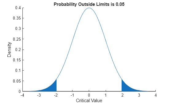
Figure contains an axes object. The axes object with title Probability Outside Limits is 0.05, xlabel Critical Value, ylabel Density contains 5 objects of type line, patch.

p = 0.0500

Input Arguments

collapse all

Probability distribution name, specified as one of the probability distribution names in this table.

nameDistributionInput Parameter AInput Parameter BInput Parameter CInput Parameter D
'Beta'Beta Distributiona first shape parameterb second shape parameterN/AN/A
'Binomial'Binomial Distributionn number of trialsp probability of success for each trialN/AN/A
'BirnbaumSaunders'Birnbaum-Saunders Distributionβ scale parameterγ shape parameterN/AN/A
'Burr'Burr Type XII Distributionα scale parameterc first shape parameterk second shape parameterN/A
'Chisquare' or 'chi2'Chi-Square Distributionν degrees of freedomN/AN/AN/A
'Exponential'Exponential Distributionμ meanN/AN/AN/A
'Extreme Value' or 'ev'Extreme Value Distributionμ location parameterσ scale parameterN/AN/A
'F'F Distributionν1 numerator degrees of freedomν2 denominator degrees of freedomN/AN/A
'Gamma'Gamma Distributiona shape parameterb scale parameterN/AN/A
'Generalized Extreme Value' or 'gev'Generalized Extreme Value Distributionk shape parameterσ scale parameterμ location parameterN/A
'Generalized Pareto' or 'gp'Generalized Pareto Distributionk tail index (shape) parameterσ scale parameterμ threshold (location) parameterN/A
'Geometric'Geometric Distributionp probability parameterN/AN/AN/A
'Half Normal' or 'hn'Half-Normal Distributionμ location parameterσ scale parameterN/AN/A
'Hypergeometric' or 'hyge'Hypergeometric Distributionm size of the populationk number of items with the desired characteristic in the populationn number of samples drawnN/A
'InverseGaussian'Inverse Gaussian Distributionμ scale parameterλ shape parameterN/AN/A
'Logistic'Logistic Distributionμ meanσ scale parameterN/AN/A
'LogLogistic'Loglogistic Distributionμ mean of logarithmic valuesσ scale parameter of logarithmic valuesN/AN/A
'LogNormal'Lognormal Distributionμ mean of logarithmic valuesσ standard deviation of logarithmic valuesN/AN/A
'Loguniform'Loguniform Distributiona lower endpoint (minimum)b upper endpoint (maximum)N/AN/A
'Nakagami'Nakagami Distributionμ shape parameterω scale parameterN/AN/A
'Negative Binomial' or 'nbin'Negative Binomial Distributionr number of successesp probability of success in a single trialN/AN/A
'Noncentral F' or 'ncf'Noncentral F Distributionν1 numerator degrees of freedomν2 denominator degrees of freedomδ noncentrality parameterN/A
'Noncentral t' or 'nct'Noncentral t Distributionν degrees of freedomδ noncentrality parameterN/AN/A
'Noncentral Chi-square' or 'ncx2'Noncentral Chi-Square Distributionν degrees of freedomδ noncentrality parameterN/AN/A
'Normal'Normal Distributionμ mean σ standard deviationN/AN/A
'Poisson'Poisson Distributionλ meanN/AN/AN/A
'Rayleigh'Rayleigh Distributionb scale parameterN/AN/AN/A
'Rician'Rician Distributions noncentrality parameterσ scale parameterN/AN/A
'Stable'Stable Distributionα first shape parameterβ second shape parameterγ scale parameterδ location parameter
'T'Student's t Distributionν degrees of freedomN/AN/AN/A
'tLocationScale't Location-Scale Distributionμ location parameterσ scale parameterν shape parameterN/A
'Uniform'Uniform Distribution (Continuous)a lower endpoint (minimum)b upper endpoint (maximum)N/AN/A
'Discrete Uniform' or 'unid'Uniform Distribution (Discrete)n maximum observable valueN/AN/AN/A
'Weibull' or 'wbl'Weibull Distributiona scale parameterb shape parameterN/AN/A

Example: 'Normal'

Probability values at which to evaluate the icdf, specified as a scalar value, or an array of scalar values in the range [0,1].

If one or more of the input arguments p, A, B, C, and D are arrays, then the array sizes must be the same. In this case, icdf expands each scalar input into a constant array of the same size as the array inputs. See name for the definitions of A, B, C, and D for each distribution.

Example: [0.1,0.25,0.5,0.75,0.9]

Data Types: single | double

First probability distribution parameter, specified as a scalar value or an array of scalar values.

If one or more of the input arguments p, A, B, C, and D are arrays, then the array sizes must be the same. In this case, icdf expands each scalar input into a constant array of the same size as the array inputs. See name for the definitions of A, B, C, and D for each distribution.

Data Types: single | double

Second probability distribution parameter, specified as a scalar value or an array of scalar values.

If one or more of the input arguments p, A, B, C, and D are arrays, then the array sizes must be the same. In this case, icdf expands each scalar input into a constant array of the same size as the array inputs. See name for the definitions of A, B, C, and D for each distribution.

Data Types: single | double

Third probability distribution parameter, specified as a scalar value or an array of scalar values.

If one or more of the input arguments p, A, B, C, and D are arrays, then the array sizes must be the same. In this case, icdf expands each scalar input into a constant array of the same size as the array inputs. See name for the definitions of A, B, C, and D for each distribution.

Data Types: single | double

Fourth probability distribution parameter, specified as a scalar value or an array of scalar values.

If one or more of the input arguments p, A, B, C, and D are arrays, then the array sizes must be the same. In this case, icdf expands each scalar input into a constant array of the same size as the array inputs. See name for the definitions of A, B, C, and D for each distribution.

Data Types: single | double

Probability distribution, specified as one of the probability distribution objects in this table.

Distribution ObjectFunction or App to Create Probability Distribution Object
BetaDistributionmakedist, fitdist, Distribution Fitter
BinomialDistributionmakedist, fitdist, Distribution Fitter
BirnbaumSaundersDistributionmakedist, fitdist, Distribution Fitter
BurrDistributionmakedist, fitdist, Distribution Fitter
ExponentialDistributionmakedist, fitdist, Distribution Fitter
ExtremeValueDistributionmakedist, fitdist, Distribution Fitter
GammaDistributionmakedist, fitdist, Distribution Fitter
GeneralizedExtremeValueDistributionmakedist, fitdist, Distribution Fitter
GeneralizedParetoDistributionmakedist, fitdist, Distribution Fitter
HalfNormalDistributionmakedist, fitdist, Distribution Fitter
InverseGaussianDistributionmakedist, fitdist, Distribution Fitter
KernelDistributionfitdist, Distribution Fitter
LogisticDistributionmakedist, fitdist, Distribution Fitter
LoglogisticDistributionmakedist, fitdist, Distribution Fitter
LognormalDistributionmakedist, fitdist, Distribution Fitter
LoguniformDistributionmakedist
MultinomialDistributionmakedist
NakagamiDistributionmakedist, fitdist, Distribution Fitter
NegativeBinomialDistributionmakedist, fitdist, Distribution Fitter
NormalDistributionmakedist, fitdist, Distribution Fitter
Piecewise distribution with generalized Pareto distributions in the tailsparetotails
PiecewiseLinearDistributionmakedist
PoissonDistributionmakedist, fitdist, Distribution Fitter
RayleighDistributionmakedist, fitdist, Distribution Fitter
RicianDistributionmakedist, fitdist, Distribution Fitter
StableDistributionmakedist, fitdist, Distribution Fitter
tLocationScaleDistributionmakedist, fitdist, Distribution Fitter
TriangularDistributionmakedist
UniformDistributionmakedist
WeibullDistributionmakedist, fitdist, Distribution Fitter

Output Arguments

collapse all

icdf values, returned as a scalar value or an array of scalar values. x is the same size as p after any necessary scalar expansion. Each element in x is the icdf value of the distribution, specified by the corresponding elements in the distribution parameters (A, B, C, and D) or specified by the probability distribution object (pd), evaluated at the corresponding element in p.

Alternative Functionality

icdf is a generic function that accepts either a distribution by its name name or a probability distribution object pd. It is faster to use a distribution-specific function, such as norminv for the normal distribution and binoinv for the binomial distribution. For a list of distribution-specific functions, see Supported Distributions.

Extended Capabilities

Version History

Introduced before R2006a