occlusionSensitivity
Explain network predictions by occluding the inputs
Description
scoreMap = occlusionSensitivity(net,X,channelIdx)X are occluded with a mask. The change in score is relative to
the original data without occlusion. The occluding mask is moved across the input data,
giving a change in score for each mask location. Use an occlusion sensitivity map to
identify the parts of your input data that most impact the score. Areas in the map with
higher positive values correspond to regions of input data that contribute positively to the
specified channel index. For classification tasks, specify the
channelIdx as the channel in the softmax layer corresponding to the
class label of interest.
___ = occlusionSensitivity(___,
specifies options using one or more name-value arguments in addition to the input arguments
in previous syntaxes. For example, Name=Value)Stride=50 sets the stride of the
occluding mask to 50 pixels.
Examples
Load a pretrained GoogLeNet network and the corresponding class names. This requires the Deep Learning Toolbox™ Model for GoogLeNet Network support package. If this support package is not installed, then the software provides a download link. For a list of all available networks, see Pretrained Deep Neural Networks.
[net,classNames] = imagePretrainedNetwork("googlenet");Import the image and resize to match the input size for the network.
X = imread("sherlock.jpg");

inputSize = net.Layers(1).InputSize(1:2);
X = imresize(X,inputSize);
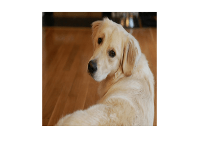
Display the image.
imshow(X)

Classify the image. To make prediction with a single observation, use the predict function. To convert the prediction scores to labels, use the scores2label function. To use a GPU, first convert the data to gpuArray. Using a GPU requires a Parallel Computing Toolbox™ license and a supported GPU device. For information on supported devices, see GPU Computing Requirements (Parallel Computing Toolbox).
if canUseGPU
    X = gpuArray(X);
end
scores = predict(net,single(X));
[label,score] = scores2label(scores,classNames);
Use occlusionSensitivity to determine which parts of the image positively influence the classification result.
channel = find(string(label) == classNames);
scoreMap = occlusionSensitivity(net,X,channel);
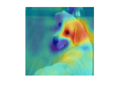
Plot the result over the original image with transparency to see which areas of the image affect the classification score.
figure
imshow(X)
hold on
imagesc(scoreMap,'AlphaData',0.5);
colormap jet

The red parts of the map show the areas which have a positive contribution to the specified label. The dog's left eye and ear strongly influence the network's prediction of golden retriever.
You can get similar results using the gradient class activation mapping (Grad-CAM) technique. Grad-CAM uses the gradient of the classification score with respect to the last convolutional layer in a network in order to understand which parts of the image are most important for classification. For an example, see Grad-CAM Reveals the Why Behind Deep Learning Decisions.
Input Arguments
Trained network, specified as a dlnetwork object.
net must contain a single input layer. The input layer must be an imageInputLayer.
Input image, specified as a numeric array.
The image must be the same size as the image input size of the network
net. The input size is specified by the
InputSize property of the imageInputLayer in the network.
Data Types: single | double | int8 | int16 | int32 | int64 | uint8 | uint16 | uint32 | uint64
Channel index, specified as a scalar or a vector of channel indices. The possible
choices for channelIdx depend on the selected layer. The function
computes the scores using the layer specified by the OutputNames
property of the dlnetwork object net and the channel
specified by channelIdx.
If channelIdx is specified as a vector, the feature importance
map for each specified channel is calculated independently. In that case,
scoreMap(:,:,i) corresponds to the map for the
ith element in channelIdx.
Data Types: single | double | int8 | int16 | int32 | int64 | uint8 | uint16 | uint32 | uint64
Name-Value Arguments
Specify optional pairs of arguments as
Name1=Value1,...,NameN=ValueN, where Name is
the argument name and Value is the corresponding value.
Name-value arguments must appear after other arguments, but the order of the
pairs does not matter.
Example: MaskSize=75,OutputUpsampling="nearest" uses an occluding mask
with size 75 pixels along each side, and uses nearest-neighbor interpolation to upsample the
output to the same size as the input data
Size of occluding mask, specified as:
"auto"— Use a mask size of 20% of the input size, rounded to the nearest integer.A vector of the form
[h w]— Use a rectangular mask with heighthand widthw.A scalar — Use a square mask with height and width equal to the specified value.
Example: MaskSize=[50 60]
Step size for traversing the mask across the input data, specified as:
"auto"— Use a stride of 10% of the input size, rounded to the nearest integer.A vector of the form
[a b]— Use a vertical stride ofaand a horizontal stride ofb.A scalar — Use a stride of the specified value in both the vertical and horizontal directions.
Example: Stride=30
Replacement value of occluded region, specified as:
"auto"— Replace occluded pixels with the channel-wise mean of the input data.A scalar — Replace occluded pixels with the specified value.
A vector — Replace occluded pixels with the value specified for each channel. The vector must contain the same number of elements as the number of output channels of the layer.
Example: MaskValue=0.5
Output upsampling method, specified as:
"bicubic"— Use bicubic interpolation to produce a smooth map the same size as the input data."nearest"— Use nearest-neighbor interpolation to resize the map to have the same resolution as the input data."none"— Use no upsampling. The map can be smaller than the input data.
If OutputUpsampling is "bicubic" or "nearest", the computed map is upsampled to the size of the input data using the imresize function.
Example: OutputUpsampling="none"
Edge handling of the occluding mask, specified as:
"on"— Place the center of the first mask at the top-left corner of the input data. Masks at the edges of the data are not full size."off"— Place the top-left corner of the first mask at the top-left corner of the input data. Masks are always full size. If the values of theMaskSizeandStrideoptions mean that some masks extend past the boundaries of the data, those masks are excluded.
For non-image input data, you can ensure you always occlude the same amount of
input data using the option by specifying MaskClipping as
"off". For example, for word embeddings data, you can ensure the
same number of words are occluded at each point.
Example: MaskClipping="off"
Size of the mini-batch to use to compute the score map, specified as a positive integer.
The mini-batch size specifies the number of images that are passed to the network at once. Larger mini-batch sizes lead to faster computation, at the cost of more memory.
Example: MiniBatchSize=256
Hardware resource, specified as one of these values:
"auto"— Use a GPU if one is available. Otherwise, use the CPU."gpu"— Use the GPU. Using a GPU requires a Parallel Computing Toolbox™ license and a supported GPU device. For information about supported devices, see GPU Computing Requirements (Parallel Computing Toolbox). If Parallel Computing Toolbox or a suitable GPU is not available, then the software returns an error."cpu"— Use the CPU.
Output Arguments
Map of change of total activation, returned as a numeric array.
The function computes the change in total activation due to occlusion. The total activation is computed by summing over all spatial dimensions of the activation of that channel. The occlusion sensitivity map corresponds to the difference between the total activation of the original data with no occlusion and the total activation for the occluded data. Areas in the map with higher positive values correspond to regions of input data that contribute positively to the specified channel activation.
If channelIdx is specified as a vector, then the change in total
activation for each specified channel is calculated independently. In that case,
scoreMap(:,:,i) corresponds to the occlusion sensitivity map for
the ith element in channel.
Extended Capabilities
The occlusionSensitivity function fully supports GPU acceleration.
By default, occlusionSensitivity uses a GPU if one is available. You can specify
the hardware that the occlusionSensitivity function uses by specifying the
ExecutionEnvironment name-value argument.
For more information, see Run MATLAB Functions on a GPU (Parallel Computing Toolbox).
Version History
Introduced in R2019b
DAGNetwork and SeriesNetwork objects are not recommended.
Use dlnetwork objects instead.
The syntax scoreMap = occlusionSensitivity(net,X,label) is supported for
DAGNetwork and SeriesNetwork objects only, where
label is the class label used to calculate change in classification
score, specified as a categorical, a character array, or a string array. To use a
dlnetwork object with the occlusionSensitivity function, you
must specify the channel index instead. To find the channel index, you must know the order of
the classes that the network was trained on.
Use the trainnet function to create a dlnetwork object. To convert an existing DAGNetwork or SeriesNetwork object to a dlnetwork object, use the dag2dlnetwork function.
This table shows how to convert code that uses a DAGNetwork object to
code that uses a dlnetwork object. You can use the same syntaxes to convert
a SeriesNetwork object.
Not recommended (DAGNetwork object) | Recommended (dlnetwork object) |
|---|---|
map = occlusionSensitivity(DAGnet,X,label); | net = dag2dlnetwork(DAGnet); channelIdx = find(label == classNames); map = occlusionSensitivity(net,X,channelIdx); classNames
contains the classes on which the network was trained. For example, you can
extract the class names from a trained classification
DAGNetwork using this
code:classNames = DAGnet.Layers(end).Classes; |
map = occlusionSensitivity(DAGnet,X,layerName,channelIdx); | To compute the map, the net = dag2dlnetwork(DAGnet); net.OutputNames = layerName; map = occlusionSensitivity(net,X,channelIdx); |
Starting in R2024a, you can use the occlusionSensitivity function to generate scores maps for nonclassification tasks, such as regression.
See Also
dlnetwork | testnet | minibatchpredict | scores2label | imageLIME | gradCAM | predict | forward
Topics
- Understand Network Predictions Using Occlusion
- Grad-CAM Reveals the Why Behind Deep Learning Decisions
- Understand Network Predictions Using LIME
- Investigate Network Predictions Using Class Activation Mapping
- Visualize Features of a Convolutional Neural Network
- Visualize Activations of a Convolutional Neural Network
MATLAB Command
You clicked a link that corresponds to this MATLAB command:
Run the command by entering it in the MATLAB Command Window. Web browsers do not support MATLAB commands.
Select a Web Site
Choose a web site to get translated content where available and see local events and offers. Based on your location, we recommend that you select: .
You can also select a web site from the following list
How to Get Best Site Performance
Select the China site (in Chinese or English) for best site performance. Other MathWorks country sites are not optimized for visits from your location.
Americas
- América Latina (Español)
- Canada (English)
- United States (English)
Europe
- Belgium (English)
- Denmark (English)
- Deutschland (Deutsch)
- España (Español)
- Finland (English)
- France (Français)
- Ireland (English)
- Italia (Italiano)
- Luxembourg (English)
- Netherlands (English)
- Norway (English)
- Österreich (Deutsch)
- Portugal (English)
- Sweden (English)
- Switzerland
- United Kingdom (English)