Create Simple Deep Learning Neural Network for Classification
This example shows how to create and train a simple convolutional neural network for deep learning classification.
Convolutional neural networks are essential tools for deep learning, and are especially suited for image recognition.
The example demonstrates how to:
Load and explore image data.
Define the neural network architecture.
Specify training options.
Train the neural network.
Predict the labels of new data and calculate the classification accuracy.
For an example showing how to interactively create and train a simple image classification neural network, see Get Started with Image Classification.
Load and Explore Image Data
Load the digits data as an image datastore using the imageDatastore function and specify the folder containing the image data. An image datastore enables you to store large image data, including data that does not fit in memory, and efficiently read batches of images during training of a convolutional neural network.
unzip("DigitsData.zip");
dataFolder = "DigitsData";
imds = imageDatastore(dataFolder, ...
    IncludeSubfolders=true, ...
    LabelSource="foldernames");
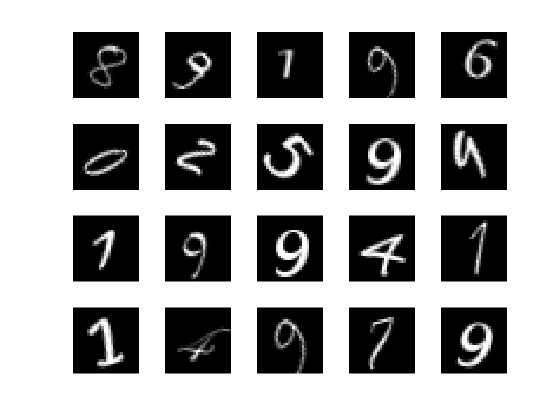
Display some of the images in the datastore.
figure
tiledlayout("flow");
perm = randperm(10000,20);
for i = 1:20
    nexttile
    imshow(imds.Files{perm(i)});
end
Calculate the number of images in each category. labelCount is a table that contains the labels and the number of images having each label. The datastore contains 1000 images for each of the digits 0-9, for a total of 10000 images. You can specify the number of classes in the last fully connected layer of your neural network as the OutputSize argument.
classNames = categories(imds.Labels);
labelCount = countEachLabel(imds)
labelCount=10×2 table
    Label    Count
    _____    _____

      0      1000
      1      1000
      2      1000
      3      1000
      4      1000
      5      1000
      6      1000
      7      1000
      8      1000
      9      1000
You must specify the size of the images in the input layer of the neural network. Check the size of the first image in digitData. Each image is 28-by-28-by-1 pixels.
img = readimage(imds,1);
size(img)
ans = 1×2

    28    28
Specify Training and Validation Sets
Divide the data into training and validation data sets, so that each category in the training set contains 750 images, and the validation set contains the remaining images from each label. splitEachLabel splits the datastore imds into two new datastores, imdsTrain and imdsValidation.
numTrainFiles = 750;
[imdsTrain,imdsValidation] = splitEachLabel(imds,numTrainFiles,"randomize");
Define Neural Network Architecture
Define the convolutional neural network architecture.
layers = [
    imageInputLayer([28 28 1])

    convolution2dLayer(3,8,Padding="same")
    batchNormalizationLayer
    reluLayer

    maxPooling2dLayer(2,Stride=2)

    convolution2dLayer(3,16,Padding="same")
    batchNormalizationLayer
    reluLayer

    maxPooling2dLayer(2,Stride=2)

    convolution2dLayer(3,32,Padding="same")
    batchNormalizationLayer
    reluLayer

    fullyConnectedLayer(10)
    softmaxLayer];
Image Input Layer An imageInputLayer is where you specify the image size, which, in this case, is 28-by-28-by-1. These numbers correspond to the height, width, and the channel size. The digit data consists of grayscale images, so the channel size (color channel) is 1. For a color image, the channel size is 3, corresponding to the RGB values. You do not need to shuffle the data because trainnet, by default, shuffles the data at the beginning of training. trainnet can also automatically shuffle the data at the beginning of every epoch during training.
Convolutional Layer In the convolutional layer, the first argument is filterSize, which is the height and width of the filters the training function uses while scanning along the images. In this example, the number 3 indicates that the filter size is 3-by-3. You can specify different sizes for the height and width of the filter. The second argument is the number of filters, numFilters, which is the number of neurons that connect to the same region of the input. This parameter determines the number of feature maps. Use the Padding name-value argument to add padding to the input feature map. For a convolutional layer with a default stride of 1, "same" padding ensures that the spatial output size is the same as the input size. You can also define the stride and learning rates for this layer using name-value arguments of convolution2dLayer.
Batch Normalization Layer Batch normalization layers normalize the activations and gradients propagating through a neural network, making neural network training an easier optimization problem. Use batch normalization layers between convolutional layers and nonlinearities, such as ReLU layers, to speed up neural network training and reduce the sensitivity to neural network initialization. Use batchNormalizationLayer to create a batch normalization layer.
ReLU Layer The batch normalization layer is followed by a nonlinear activation function. The most common activation function is the rectified linear unit (ReLU). Use reluLayer to create a ReLU layer.
Max Pooling Layer Convolutional layers (with activation functions) are sometimes followed by a down-sampling operation that reduces the spatial size of the feature map and removes redundant spatial information. Down-sampling makes it possible to increase the number of filters in deeper convolutional layers without increasing the required amount of computation per layer. One way of down-sampling is using a max pooling, which you create using maxPooling2dLayer. The max pooling layer returns the maximum values of rectangular regions of inputs, specified by the first argument, poolSize. In this example, the size of the rectangular region is [2,2]. The Stride name-value argument specifies the step size that the training function takes as it scans along the input.
Fully Connected Layer The convolutional and down-sampling layers are followed by one or more fully connected layers. As its name suggests, a fully connected layer is a layer in which the neurons connect to all the neurons in the preceding layer. This layer combines all the features learned by the previous layers across the image to identify the larger patterns. The last fully connected layer combines the features to classify the images. Therefore, the OutputSize parameter in the last fully connected layer is equal to the number of classes in the target data. In this example, the output size is 10, corresponding to the 10 classes. Use fullyConnectedLayer to create a fully connected layer.
Softmax Layer The softmax activation function normalizes the output of the fully connected layer. The output of the softmax layer consists of positive numbers that sum to one, which can then be used as classification probabilities by the classification layer. Create a softmax layer using the softmaxLayer function after the last fully connected layer.
Specify Training Options
Specify the training options. Choosing among the options requires empirical analysis. To explore different training option configurations by running experiments, you can use the Experiment Manager app.
Train the neural network using stochastic gradient descent with momentum (SGDM) with an initial learning rate of 0.01.
Set the maximum number of epochs to 4. An epoch is a full training cycle on the entire training data set.
Shuffle the data every epoch.
Monitor the neural network accuracy during training by specifying validation data and validation frequency. The software trains the neural network on the training data and calculates the accuracy on the validation data at regular intervals during training. The validation data is not used to update the neural network weights.
Display the training progress in a plot and monitor the accuracy.
Disable the verbose output.
options = trainingOptions("sgdm", ...
    InitialLearnRate=0.01, ...
    MaxEpochs=4, ...
    Shuffle="every-epoch", ...
    ValidationData=imdsValidation, ...
    ValidationFrequency=30, ...
    Plots="training-progress", ...
    Metrics="accuracy", ...
    Verbose=false);
Train Neural Network Using Training Data
Train the neural network using the architecture defined by layers, the training data, and the training options. By default, trainnet uses a GPU if one is available, otherwise, it uses a CPU. Training on a GPU requires Parallel Computing Toolbox™ and a supported GPU device. For information on supported devices, see GPU Computing Requirements (Parallel Computing Toolbox). You can also specify the execution environment by using the ExecutionEnvironment name-value argument of trainingOptions.
The training progress plot shows the mini-batch loss and accuracy and the validation loss and accuracy. For more information on the training progress plot, see Monitor Deep Learning Training Progress. The loss is the cross-entropy loss. The accuracy is the percentage of images that the neural network classifies correctly.
net = trainnet(imdsTrain,layers,"crossentropy",options);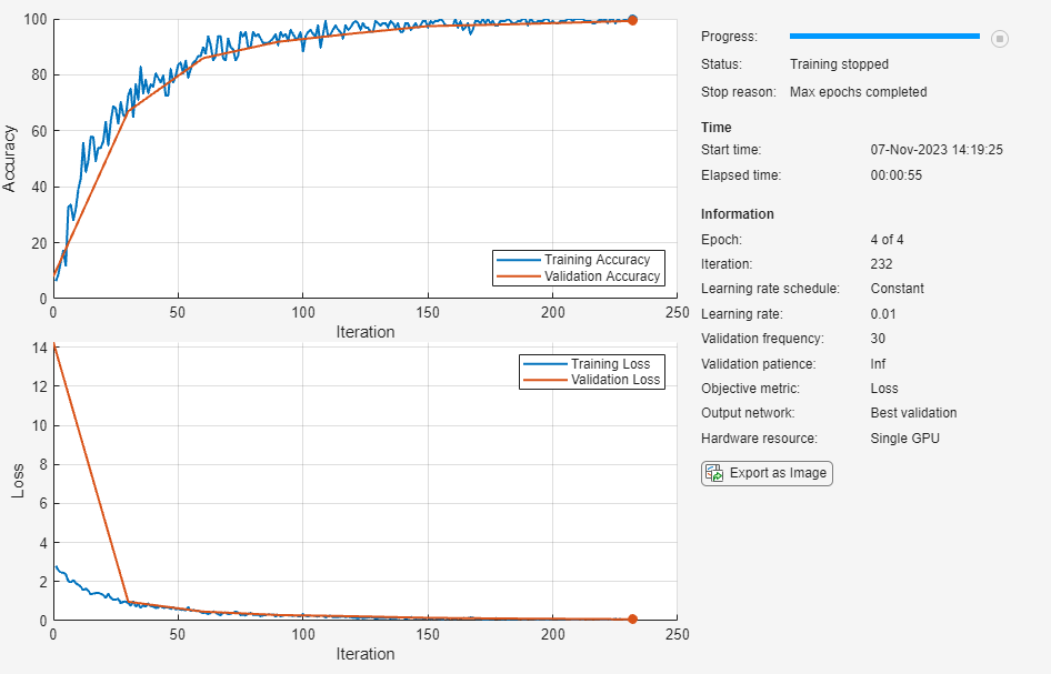
Classify Validation Images and Compute Accuracy
Classify the test images. To make predictions with multiple observations, use the minibatchpredict function. To convert the prediction scores to labels, use the scores2label function. The minibatchpredict function automatically uses a GPU if one is available. Otherwise, the function uses the CPU.
scores = minibatchpredict(net,imdsValidation);
YValidation = scores2label(scores,classNames);
Calculate the classification accuracy. The accuracy is the percentage of correctly predicted labels.
TValidation = imdsValidation.Labels;
accuracy = mean(YValidation == TValidation)
accuracy = 0.9928
See Also
trainnet | trainingOptions | dlnetwork | analyzeNetwork | Deep Network
Designer