Deep Learning Using Bayesian Optimization
This example shows how to apply Bayesian optimization to deep learning and find optimal network hyperparameters and training options for convolutional neural networks.
To train a deep neural network, you must specify the neural network architecture, as well as options of the training algorithm. Selecting and tuning these hyperparameters can be difficult and take time. Bayesian optimization is an algorithm well suited to optimizing hyperparameters of classification and regression models. You can use Bayesian optimization to optimize functions that are nondifferentiable, discontinuous, and time-consuming to evaluate. The algorithm internally maintains a Gaussian process model of the objective function, and uses objective function evaluations to train this model.
This example shows how to:
Download and prepare the CIFAR-10 data set for network training. This data set is one of the most widely used data sets for testing image classification models.
Specify variables to optimize using Bayesian optimization. These variables are options of the training algorithm, as well as parameters of the network architecture itself.
Define the objective function, which takes the values of the optimization variables as inputs, specifies the network architecture and training options, trains and validates the network, and saves the trained network to disk. The objective function is defined at the end of this script.
Perform Bayesian optimization by minimizing the classification error on the validation set.
Load the best network from disk and evaluate it on the test set.
As an alternative, you can use Bayesian optimization to find optimal training options in Experiment Manager. For more information, see Tune Experiment Hyperparameters by Using Bayesian Optimization.
Prepare Data
Download the CIFAR-10 data set [1]. This data set contains 60,000 images, and each image has the size 32-by-32 and three color channels (RGB). The size of the whole data set is 175 MB. Depending on your internet connection, the download process can take some time.
datadir = tempdir;
downloadCIFARData(datadir);
Load the CIFAR-10 data set as training images and labels, and test images and labels. To enable network validation, use 5000 of the test images for validation.
[XTrain,YTrain,XTest,YTest] = loadCIFARData(datadir);

idx = randperm(numel(YTest),5000);
XValidation = XTest(:,:,:,idx);
XTest(:,:,:,idx) = [];
YValidation = YTest(idx);
YTest(idx) = [];
You can display a sample of the training images using the following code.
figure;
idx = randperm(numel(YTrain),20);
for i = 1:numel(idx)
    subplot(4,5,i);
    imshow(XTrain(:,:,:,idx(i)));
end
Choose Variables to Optimize
Choose which variables to optimize using Bayesian optimization, and specify the ranges to search in. Also, specify whether the variables are integers and whether to search the interval in logarithmic space. Optimize the following variables:
Network section depth. This parameter controls the depth of the network. The network has three sections, each with
SectionDepthidentical convolutional layers. So the total number of convolutional layers is3*SectionDepth. The objective function later in the script takes the number of convolutional filters in each layer proportional to1/sqrt(SectionDepth). As a result, the number of parameters and the required amount of computation for each iteration are roughly the same for different section depths.Initial learning rate. The best learning rate can depend on your data as well as the network you are training.
Stochastic gradient descent momentum. Momentum adds inertia to the parameter updates by having the current update contain a contribution proportional to the update in the previous iteration. This results in more smooth parameter updates and a reduction of the noise inherent to stochastic gradient descent.
L2 regularization strength. Use regularization to prevent overfitting. Search the space of regularization strength to find a good value. Data augmentation and batch normalization also help regularize the network.
optimVars = [
    optimizableVariable('SectionDepth',[1 3],'Type','integer')
    optimizableVariable('InitialLearnRate',[1e-2 1],'Transform','log')
    optimizableVariable('Momentum',[0.8 0.98])
    optimizableVariable('L2Regularization',[1e-10 1e-2],'Transform','log')];
Perform Bayesian Optimization
Create the objective function for the Bayesian optimizer, using the training and validation data as inputs. The objective function trains a convolutional neural network and returns the classification error on the validation set. This function is defined at the end of this script. Because bayesopt uses the error rate on the validation set to choose the best model, it is possible that the final network overfits on the validation set. The final chosen model is then tested on the independent test set to estimate the generalization error.
ObjFcn = makeObjFcn(XTrain,YTrain,XValidation,YValidation);
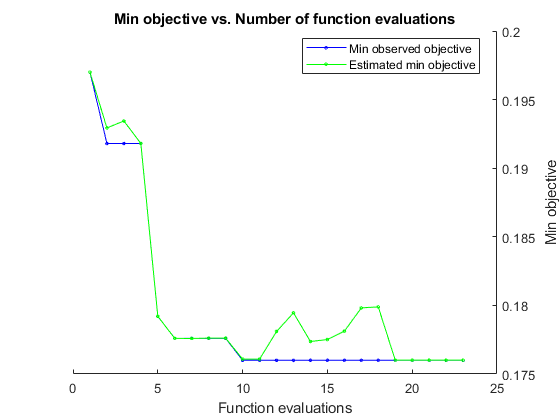
Perform Bayesian optimization by minimizing the classification error on the validation set. Specify the total optimization time in seconds. To best utilize the power of Bayesian optimization, you should perform at least 30 objective function evaluations. To train networks in parallel on multiple GPUs, set the 'UseParallel' value to true. If you have a single GPU and set the 'UseParallel' value to true, then all workers share that GPU, and you obtain no training speed-up and increase the chances of the GPU running out of memory.
After each network finishes training, bayesopt prints the results to the command window. The bayesopt function then returns the file names in BayesObject.UserDataTrace. The objective function saves the trained networks to disk and returns the file names to bayesopt.
BayesObject = bayesopt(ObjFcn,optimVars, ...
    'MaxTime',14*60*60, ...
    'IsObjectiveDeterministic',false, ...
    'UseParallel',false);
|===================================================================================================================================|
| Iter | Eval   | Objective   | Objective   | BestSoFar   | BestSoFar   | SectionDepth | InitialLearn-|     Momentum | L2Regulariza-|
|      | result |             | runtime     | (observed)  | (estim.)    |              | Rate         |              | tion         |
|===================================================================================================================================|
|    1 | Best   |       0.197 |      955.69 |       0.197 |       0.197 |            3 |      0.61856 |      0.80624 |   0.00035179 |
| 2 | Best | 0.1918 | 790.38 | 0.1918 | 0.19293 | 2 | 0.074118 | 0.91031 | 2.7229e-09 |
| 3 | Accept | 0.2438 | 660.29 | 0.1918 | 0.19344 | 1 | 0.051153 | 0.90911 | 0.00043113 |
| 4 | Accept | 0.208 | 672.81 | 0.1918 | 0.1918 | 1 | 0.70138 | 0.81923 | 3.7783e-08 |
| 5 | Best | 0.1792 | 844.07 | 0.1792 | 0.17921 | 2 | 0.65156 | 0.93783 | 3.3663e-10 |
| 6 | Best | 0.1776 | 851.49 | 0.1776 | 0.17759 | 2 | 0.23619 | 0.91932 | 1.0007e-10 |
| 7 | Accept | 0.2232 | 883.5 | 0.1776 | 0.17759 | 2 | 0.011147 | 0.91526 | 0.0099842 |
| 8 | Accept | 0.2508 | 822.65 | 0.1776 | 0.17762 | 1 | 0.023919 | 0.91048 | 1.0002e-10 |
| 9 | Accept | 0.1974 | 1947.6 | 0.1776 | 0.17761 | 3 | 0.010017 | 0.97683 | 5.4603e-10 |
| 10 | Best | 0.176 | 1938.4 | 0.176 | 0.17608 | 2 | 0.3526 | 0.82381 | 1.4244e-07 |
| 11 | Accept | 0.1914 | 2874.4 | 0.176 | 0.17608 | 3 | 0.079847 | 0.86801 | 9.7335e-07 |
| 12 | Accept | 0.181 | 2578 | 0.176 | 0.17809 | 2 | 0.35141 | 0.80202 | 4.5634e-08 |
| 13 | Accept | 0.1838 | 2410.8 | 0.176 | 0.17946 | 2 | 0.39508 | 0.95968 | 9.3856e-06 |
| 14 | Accept | 0.1786 | 2490.6 | 0.176 | 0.17737 | 2 | 0.44857 | 0.91827 | 1.0939e-10 |
| 15 | Accept | 0.1776 | 2668 | 0.176 | 0.17751 | 2 | 0.95793 | 0.85503 | 1.0222e-05 |
| 16 | Accept | 0.1824 | 3059.8 | 0.176 | 0.17812 | 2 | 0.41142 | 0.86931 | 1.447e-06 |
| 17 | Accept | 0.1894 | 3091.5 | 0.176 | 0.17982 | 2 | 0.97051 | 0.80284 | 1.5836e-10 |
| 18 | Accept | 0.217 | 2794.5 | 0.176 | 0.17989 | 1 | 0.2464 | 0.84428 | 4.4938e-06 |
| 19 | Accept | 0.2358 | 4054.2 | 0.176 | 0.17601 | 3 | 0.22843 | 0.9454 | 0.00098248 |
| 20 | Accept | 0.2216 | 4411.7 | 0.176 | 0.17601 | 3 | 0.010847 | 0.82288 | 2.4756e-08 |
|===================================================================================================================================|
| Iter | Eval   | Objective   | Objective   | BestSoFar   | BestSoFar   | SectionDepth | InitialLearn-|     Momentum | L2Regulariza-|
|      | result |             | runtime     | (observed)  | (estim.)    |              | Rate         |              | tion         |
|===================================================================================================================================|
|   21 | Accept |      0.2038 |      3906.4 |       0.176 |     0.17601 |            2 |      0.09885 |      0.81541 |    0.0021184 |
| 22 | Accept | 0.2492 | 4103.4 | 0.176 | 0.17601 | 2 | 0.52313 | 0.83139 | 0.0016269 |
| 23 | Accept | 0.1814 | 4240.5 | 0.176 | 0.17601 | 2 | 0.29506 | 0.84061 | 6.0203e-10 |
__________________________________________________________
Optimization completed.
MaxTime of 50400 seconds reached.
Total function evaluations: 23
Total elapsed time: 53088.5123 seconds
Total objective function evaluation time: 53050.7026

Best observed feasible point:
    SectionDepth    InitialLearnRate    Momentum    L2Regularization
    ____________    ________________    ________    ________________

         2               0.3526         0.82381        1.4244e-07

Observed objective function value = 0.176
Estimated objective function value = 0.17601
Function evaluation time = 1938.4483

Best estimated feasible point (according to models):
    SectionDepth    InitialLearnRate    Momentum    L2Regularization
    ____________    ________________    ________    ________________

         2               0.3526         0.82381        1.4244e-07

Estimated objective function value = 0.17601
Estimated function evaluation time = 1898.2641
Evaluate Final Network
Load the best network found in the optimization and its validation accuracy.
bestIdx = BayesObject.IndexOfMinimumTrace(end);
fileName = BayesObject.UserDataTrace{bestIdx};
savedStruct = load(fileName);
valError = savedStruct.valError
valError = 0.1760
Predict the labels of the test set and calculate the test error. Treat the classification of each image in the test set as independent events with a certain probability of success, which means that the number of incorrectly classified images follows a binomial distribution. Use this to calculate the standard error (testErrorSE) and an approximate 95% confidence interval (testError95CI) of the generalization error rate. This method is often called the Wald method. bayesopt determines the best network using the validation set without exposing the network to the test set. It is then possible that the test error is higher than the validation error.
[YPredicted,probs] = classify(savedStruct.trainedNet,XTest);
testError = 1 - mean(YPredicted == YTest)
testError = 0.1910
NTest = numel(YTest);
testErrorSE = sqrt(testError*(1-testError)/NTest);
testError95CI = [testError - 1.96*testErrorSE, testError + 1.96*testErrorSE]
testError95CI = 1×2

    0.1801    0.2019
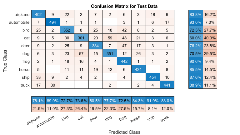
Plot the confusion matrix for the test data. Display the precision and recall for each class by using column and row summaries.
figure('Units','normalized','Position',[0.2 0.2 0.4 0.4]);
cm = confusionchart(YTest,YPredicted);
cm.Title = 'Confusion Matrix for Test Data';
cm.ColumnSummary = 'column-normalized';
cm.RowSummary = 'row-normalized';
You can display some test images together with their predicted classes and the probabilities of those classes using the following code.
figure
idx = randperm(numel(YTest),9);
for i = 1:numel(idx)
    subplot(3,3,i)
    imshow(XTest(:,:,:,idx(i)));
    prob = num2str(100*max(probs(idx(i),:)),3);
    predClass = char(YPredicted(idx(i)));
    label = [predClass,', ',prob,'%'];
    title(label)
end
Objective Function for Optimization
Define the objective function for optimization. This function performs the following steps:
Takes the values of the optimization variables as inputs.
bayesoptcalls the objective function with the current values of the optimization variables in a table with each column name equal to the variable name. For example, the current value of the network section depth isoptVars.SectionDepth.Defines the network architecture and training options.
Trains and validates the network.
Saves the trained network, the validation error, and the training options to disk.
Returns the validation error and the file name of the saved network.
function ObjFcn = makeObjFcn(XTrain,YTrain,XValidation,YValidation)
ObjFcn = @valErrorFun;
    function [valError,cons,fileName] = valErrorFun(optVars)
Define the convolutional neural network architecture.
Add padding to the convolutional layers so that the spatial output size is always the same as the input size.
Each time you downsample the spatial dimensions by a factor of two using max pooling layers, increase the number of filters by a factor of two. Doing so ensures that the amount of computation required in each convolutional layer is roughly the same.
Choose the number of filters proportional to
1/sqrt(SectionDepth), so that networks of different depths have roughly the same number of parameters and require about the same amount of computation per iteration. To increase the number of network parameters and the overall network flexibility, increasenumF. To train even deeper networks, change the range of theSectionDepthvariable.Use
convBlock(filterSize,numFilters,numConvLayers)to create a block ofnumConvLayersconvolutional layers, each with a specifiedfilterSizeandnumFiltersfilters, and each followed by a batch normalization layer and a ReLU layer. TheconvBlockfunction is defined at the end of this example.
        imageSize = [32 32 3];
        numClasses = numel(unique(YTrain));
        numF = round(16/sqrt(optVars.SectionDepth));
        layers = [
            imageInputLayer(imageSize)

            % The spatial input and output sizes of these convolutional
            % layers are 32-by-32, and the following max pooling layer
            % reduces this to 16-by-16.
            convBlock(3,numF,optVars.SectionDepth)
            maxPooling2dLayer(3,'Stride',2,'Padding','same')

            % The spatial input and output sizes of these convolutional
            % layers are 16-by-16, and the following max pooling layer
            % reduces this to 8-by-8.
            convBlock(3,2*numF,optVars.SectionDepth)
            maxPooling2dLayer(3,'Stride',2,'Padding','same')

            % The spatial input and output sizes of these convolutional
            % layers are 8-by-8. The global average pooling layer averages
            % over the 8-by-8 inputs, giving an output of size
            % 1-by-1-by-4*initialNumFilters. With a global average
            % pooling layer, the final classification output is only
            % sensitive to the total amount of each feature present in the
            % input image, but insensitive to the spatial positions of the
            % features.
            convBlock(3,4*numF,optVars.SectionDepth)
            averagePooling2dLayer(8)

            % Add the fully connected layer and the final softmax and
            % classification layers.
            fullyConnectedLayer(numClasses)
            softmaxLayer
            classificationLayer];
Specify options for network training. Optimize the initial learning rate, SGD momentum, and L2 regularization strength.
Specify validation data and choose the 'ValidationFrequency' value such that trainNetwork validates the network once per epoch. Train for a fixed number of epochs and lower the learning rate by a factor of 10 during the last epochs. This reduces the noise of the parameter updates and lets the network parameters settle down closer to a minimum of the loss function.
        miniBatchSize = 256;
        validationFrequency = floor(numel(YTrain)/miniBatchSize);
        options = trainingOptions('sgdm', ...
            'InitialLearnRate',optVars.InitialLearnRate, ...
            'Momentum',optVars.Momentum, ...
            'MaxEpochs',60, ...
            'LearnRateSchedule','piecewise', ...
            'LearnRateDropPeriod',40, ...
            'LearnRateDropFactor',0.1, ...
            'MiniBatchSize',miniBatchSize, ...
            'L2Regularization',optVars.L2Regularization, ...
            'Shuffle','every-epoch', ...
            'Verbose',false, ...
            'Plots','training-progress', ...
            'ValidationData',{XValidation,YValidation}, ...
            'ValidationFrequency',validationFrequency);
Use data augmentation to randomly flip the training images along the vertical axis, and randomly translate them up to four pixels horizontally and vertically. Data augmentation helps prevent the network from overfitting and memorizing the exact details of the training images.
        pixelRange = [-4 4];
        imageAugmenter = imageDataAugmenter( ...
            'RandXReflection',true, ...
            'RandXTranslation',pixelRange, ...
            'RandYTranslation',pixelRange);
        datasource = augmentedImageDatastore(imageSize,XTrain,YTrain,'DataAugmentation',imageAugmenter);
Train the network and plot the training progress during training. Close all training plots after training finishes.
        trainedNet = trainNetwork(datasource,layers,options);
        close(findall(groot,'Tag','NNET_CNN_TRAININGPLOT_UIFIGURE'))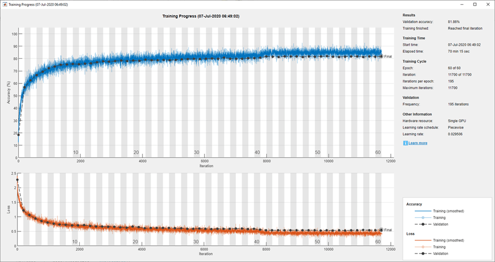
Evaluate the trained network on the validation set, calculate the predicted image labels, and calculate the error rate on the validation data.
        YPredicted = classify(trainedNet,XValidation);
        valError = 1 - mean(YPredicted == YValidation);
Create a file name containing the validation error, and save the network, validation error, and training options to disk. The objective function returns fileName as an output argument, and bayesopt returns all the file names in BayesObject.UserDataTrace. The additional required output argument cons specifies constraints among the variables. There are no variable constraints.
        fileName = num2str(valError) + ".mat";
        save(fileName,'trainedNet','valError','options')
        cons = [];

    end
end
The convBlock function creates a block of numConvLayers convolutional layers, each with a specified filterSize and numFilters filters, and each followed by a batch normalization layer and a ReLU layer.
function layers = convBlock(filterSize,numFilters,numConvLayers)
layers = [
    convolution2dLayer(filterSize,numFilters,'Padding','same')
    batchNormalizationLayer
    reluLayer];
layers = repmat(layers,numConvLayers,1);
end
References
[1] Krizhevsky, Alex. "Learning multiple layers of features from tiny images." (2009). https://www.cs.toronto.edu/~kriz/learning-features-2009-TR.pdf
See Also
Experiment
Manager | trainnet | trainingOptions | dlnetwork | bayesopt (Statistics and Machine Learning Toolbox)