Environment
Java Runtime no longer installed with MATLAB
Before R2026b, MATLAB® installations on Windows® and Linux® platforms included Java® Runtime. Starting in R2026b, MATLAB no longer includes Java as part of its installation.
You can download and install the MATLAB Support for OpenJDK® add-on or any compatible OpenJDK distribution after installing MATLAB. MATLAB continues to support OpenJDK on all platforms.
For information about supported versions, see Versions of OpenJDK Compatible with MATLAB by Release. MathWorks follows the vendors’ long-term support (LTS) guidance to determine versions for the MATLAB Support for OpenJDK add-on. Refer to the vendors’ websites for more information.
For information about changes to the jenv and matlab_jenv functions, see
Call Java from MATLAB: Install OpenJDK JRE Runtime.
Configure the desktop with more flexible layout options
You can configure the MATLAB desktop with greater layout flexibility.
Move more panels to the center of the desktop — Move the Files, Workspace, Command History, and Project panels to the center of the desktop.
Undock more panels — Undock the Debugger and Code Issues panels, allowing you to arrange them alongside an undocked Editor or Live Editor.
Reposition panels by dragging — Undock a panel or move it to the center of the desktop by dragging its title bar outside the MATLAB window or toward the center. For example, to move the Command History to the center of the desktop, drag the Command History panel title bar toward the center.
Identify and manage document groups using panel title bars — By default, documents in the center of the desktop include a title bar, which helps identify and manage document groups and panels. To show the title bar only when you hover over the edge of a document or panel tab, click the Panel actions button
 on the title bar and select Panel Headers > Show On Hover.
MATLAB also restores document locations more reliably in a session, preserving your desktop layout when you close and reopen documents.
For more information, see Configure the Desktop.
Generate and display formatted text in the Command Window
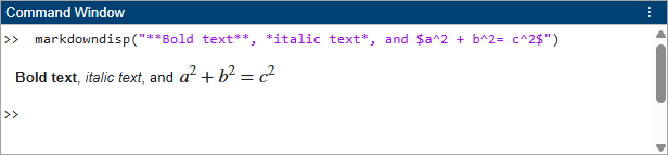
You can render Markdown text and LaTeX equations directly in the Command Window and Live
Editor using the markdowndisp
function.
For example, you can display bold and italic text and an equation.
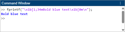
In addition, the Command Window now renders ANSI escape codes for styled and colored
text, including bold, underlined, italic, and strikethrough formatting, as well as
foreground and background colors. To display styled and colored text, use the fprintf, sprintf, or compose functions.
For example, you can display bold and blue text in the Command Window.
Large matrices are truncated in Command Window display
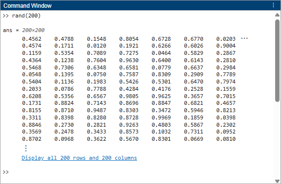
The Command Window now truncates most large two‑dimensional numeric matrices by default. To view the contents of a truncated matrix, click the link below the matrix. You also can view the contents by right-clicking the matrix or pressing Ctrl+D to open it in the Variables editor.
To disable truncating matrices by default, on the Home tab, in the Environment section, click Settings. Select MATLAB > Command Window, and in the Display section, clear the Show enhanced output (truncate matrix, render Markdown) option.
Live scripts use plain text file format by default
By default, MATLAB creates and saves live scripts and live functions using the plain text live
code file format (.m). This file format improves integration with source
control and allows you to open live code files in external text editors. Live scripts saved
in the plain text file format behave the same as other live scripts. They open in the Live
Editor and can include code, output, formatted text, interactive controls, and tasks.
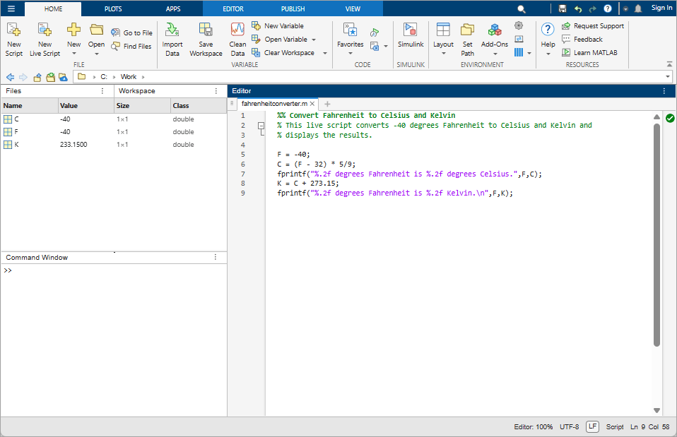
For more information, see Live Code File Formats.
Display long code lines using wrapping in the Editor
If your code file contains long code lines, the Editor or Live Editor can display those code lines across multiple visual lines without adding line breaks. This display-only wrapping helps you avoid horizontal scrolling while preserving the original code.
To enable wrapping long code lines, go to the View tab, and in the Display section, toggle the Wrap Code Lines button on. For more information, see Edit and Format Code.

Change end-of-line sequence for files open in the Editor
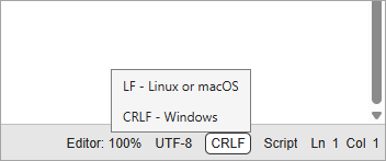
To change the end-of-line sequence for the file currently open in the Editor, click the end-of-line sequence indicator at the bottom-right corner of the MATLAB desktop and select the end-of-line sequence style to use.
For more information, see Change Line Endings.
Add variable selector to live scripts
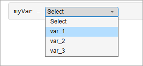
You can add a variable selector to your live script to select a workspace variable interactively. To add a variable selector, go to the Live Editor tab, and in the Code section, select Control > Variable Selector.
For more information, see Add Interactive Controls to Live Scripts.
Go to specific line and column in the Editor using improved interface
Use the improved Go To interface to navigate to a specific location in a file open in the Editor or Live Editor more quickly. To navigate to a specific location, on the Editor or Live Editor tab, in the Navigate section, select Go To > Line. Then, specify the line and optionally the column number that you want to navigate to.

Examine file and folder comparison results directly at MATLAB Command Window
You can now use the visdiff function to examine folder and file
comparison results directly at the Command Window. The comparison object now has a new
Result property that contains information such as line-by-line
comparison. For more information, see visdiff.
You can now close all currently opened comparison windows using the
comparisons.closeAll command.
Register external text merge tool
By default, to resolve merge conflicts in text-based files, MATLAB uses a built-in two-way text merge tool. You can now use an external
three-way merge tool for specific text file extensions, including .m,
.txt, and .toml. For more information, see Register External Text Merge Tool.
Functionality being removed or changed
Add-On Manager replaced by Add-Ons panel
Behavior change
The Add-On Manager has been removed. To find, install, and manage add-ons interactively, use the Add-Ons panel instead. For more information, see Get and Manage Add-Ons.
Add-on management using matlab.addons functions changed and
replaced
Behavior change in future release
These matlab.addons functions are not recommended:
There are no plans to remove the matlab.addons functions.
However, to manage add-ons, including enabling or disabling add-ons, a more efficient
approach is to uninstall and reinstall add-ons using mpminstall
and mpmuninstall, or to use MATLAB projects to manage add-on dependencies for your code. The mpmlist
function provides additional support for listing installed add-ons.
This table shows some typical uses of the matlab.addons
functions and how to update your code to use the mpminstall,
mpmuninstall, and mpmlist functions
instead.
| Not Recommended | Recommended |
|---|---|
installedAddon = matlab.addons.install("C:\Downloads\My
toolbox.mltbx") | installedAddon = mpminstall("C:\Downloads\My
toolbox.mltbx") |
installedAddon = matlab.addons.install("C:\Downloads\My
toolbox.mltbx","overwrite") | installedAddon = mpminstall("C:\Downloads\My toolbox.mltbx",
AllowVersionReplacement=true) |
installedAddon = matlab.addons.install("C:\Downloads\My
toolbox.mltbx","add") | installedAddon = mpminstall("C:\Downloads\My toolbox.mltbx",
AllowVersionReplacement=false) |
matlab.addons.uninstall("GUI Layout Toolbox")
| mpmuninstall("GUI Layout Toolbox") |
installedToolbox =
                           matlab.addons.toolbox.installToolbox("C:\Downloads\My
toolbox.mltbx") | installedToolbox = mpminstall("C:\Downloads\My
toolbox.mltbx") |
matlab.addons.toolbox.uninstallToolbox("GUI Layout Toolbox")
| mpmuninstall("GUI Layout Toolbox") |
toolboxes =
matlab.addons.toolbox.installedToolboxes | addons = mpmlist |
As part of this change, you can no longer use the agreeToLicense
argument with the matlab.addons.install and matlab.addons.toolbox.installToolbox functions to accept or review a
license agreement before installing an add-on or toolbox. License agreement approval now
occurs by default, and the license agreement and service level agreement (SLA) coverage
remain in effect, even if the license is not displayed during installation.
To view the license agreement for an add-on, go to the Add-Ons panel, and in the Installed section, click the Options button to the right of the add-on. Then, select Open Folder to open the root folder of the add-on in the Files panel, where you can access the license agreement.
In addition, when you uninstall an add-on using the matlab.addons.uninstall or matlab.addons.toolbox.uninstallToolbox functions, the add-on is removed
from the MATLAB path, but the add-on files are not removed from disk. Previously, the
add-on files were removed from disk.
Language and Programming
Validation Functions: Validate that values are scalars, vectors, or empty arrays
Use the mustBeScalar
validation function to validate that a value is a scalar. Use the mustBeVectorOrEmpty validation function to validate that a value is either a
vector or an empty array. These functions extend the existing checks
mustBeScalarOrEmpty and mustBeVector, providing
more robust size checking in function argument and property validation.
For more information, see Function Argument Validation and Property Validation Functions.
Use screen reader and keyboard to navigate Debugger panel
You can use a screen reader and keyboard shortcuts to navigate and interact with the Debugger panel. Collapse and expand files using the left and right arrow keys, enable or disable breakpoints by pressing the space bar, navigate to breakpoints by pressing Enter, and remove breakpoints by pressing Delete.
For more information about the Debugger panel, see Manage Breakpoints in Debugger Panel.
Debug code using ValidHandle property for
matlab.lang.WeakReference class
The new ValidHandle property in the matlab.lang.WeakReference class holds the same value as the
Handle property, but if they hold a reference to an invalid handle
object, MATLAB errors when you try to access ValidHandle. Use
ValidHandle to help debug your code when breaking strong reference
cycles.
Programmatically add subclasses and superclasses in Class Diagram Viewer
addSubclasses and addSuperclasses methods
The new addSubclasses and addSuperclasses methods of
matlab.diagram.ClassViewer add subclasses and superclasses, respectively, of
the specified class to the Class Browser and canvas of a Class Diagram
Viewer instance.
Warn when older class name is used after creation of new alias
WarnOnOldName is an optional name-value argument for the
addAlias method of matlab.alias.AliasFileManager. When you set WarnOnOldName to
true, MATLAB displays a warning the first time an old class name is used after creation of
a new alias.
Object Lifecycle Management: Garbage Collection (Beta)
The object lifecycle management system for MATLAB is being updated to garbage collection. The garbage collection system enables performance improvements for applications that use MATLAB objects. In particular, object creation, object deletion, and property access are faster. To try this new feature, start with this download on File Exchange. For more information about this new feature and the changes associated with it, see Object Lifecycle Management (Beta).
Note
This new feature is in beta development and should not be used for production or development activities. Software development is ongoing, and specific features are subject to change.
Functionality being removed or changed
mustBeVector(value,"allow-all-empties") syntax is not
recommended
Still runs
The validation function syntax
mustBeVector(value,"allow-all-empties") is not recommended.
Instead, use the mustBeVectorOrEmpty validation function to validate that a value is
either a vector or an empty array. You can update your code by replacing occurrences of
mustBeVector(value,"allow-all-empties") with
mustBeVectorOrEmpty(value). However, there are no plans to remove
the mustBeVector(value,"allow-all-empties") syntax.
Object that fails to load is replaced with the default object or an empty array
Behavior change
Starting in R2026b, MATLAB attempts to replace objects that fail to load under some circumstances with the default class objects. If an object cannot be replaced, MATLAB returns an empty array of the class. The new behavior applies to scalar objects and arrays of objects of non-heterogeneous classes:
Scalar objects — MATLAB attempts to call the no-argument constructor of the class to replace the object that failed to load. If this attempt fails, MATLAB returns a 0-by-1 array of the class.
Object arrays — If an element of the array fails to load, MATLAB attempts to call the no-argument constructor of the class to replace the object that failed to load and returns an array of the original size. If this attempt fails, MATLAB returns a 0-by-1 array of the class.
For example, MyClass defines Property1 of type
PropClass.
classdef MyClass
   properties
      Property1 PropClass
   end
end
If you attempt to load a saved instance of MyClass and the definition
of PropClass is not on the path, MATLAB displays a warning and returns a 0-by-1 array
of MyClass.
Deletion with logical indexing
Behavior change
When you index into an array of a built-in data type using a logical expression, MATLAB returns the array reshaped into a row vector under these conditions:
The logical indexing is used for deletion.
The logical indexing expression is false for all elements in the array.
For example, these statements return matrix doubleA reshaped into
a row vector because none of the elements are less than
0.
doubleA = ([11 22 33; 44 55 66; 77 88 99]);
doubleA(doubleA < 0) = []
doubleA =

11 44 77 22 55 88 33 66 99You can enable an optional warning to help identify code that might be affected by this change.
warning('on','MATLAB:index:allFalseLogicalDeletion')
warnStruct = warning('on','MATLAB:index:allFalseLogicalDeletion')
Compact display of handles to deleted objects
Behavior change
In compact display scenarios (cell arrays, structures, and table cells, for example), handles to deleted scalar objects now explicitly display the deleted status.
For example, create an instance of matlab.lang.HandlePlaceholder and
assign it to a field of a
structure.
obj = matlab.lang.HandlePlaceholder;
s.handleobj = obj
s =

  struct with fields:

    handleobj: [1×1 matlab.lang.HandlePlaceholder]
Delete the object and display s
again.
delete(obj)
s
s =

  struct with fields:

    handleobj: <deleted matlab.lang.HandlePlaceholder>
Before R2026b, MATLAB displayed the structure field handleobj as a 1-by-1
instance of matlab.lang.HandlePlaceholder, and you had to query the value
of s.handleobj directly to see that the handle was to a deleted
instance.
error function ignores additional fields and converts invalid
values in errorStruct.stack
Behavior change
The error function now ignores any fields in
errorStruct.stack that are not named file,
name, or line. Previously,
error preserved any additional fields in the resulting error
structure.
In addition, if the line field in
errorStruct.stack contains a noninteger value,
error uses only the real, integer part. If the
line field contains an invalid value, such as
NaN or Inf, error replaces
the value with 0. Previously, error preserved
invalid or unsupported values in the resulting error structure.
Names of classes defined using function syntax will require case-sensitive matches for folder names
Behavior change in future release
In previous releases, for classes defined using function syntax on Windows, the names of the function and the class folder did not have to be case-sensitive matches. In a future release, the names must be exact, case-sensitive matches.
Data Analysis
timetable data type supports numeric row times
Timetables now support numeric (double or single)
vectors as row times, in addition to datetime and
duration vectors. With numeric row times, you can index into
timetables by specifying unit-agnostic time or non-time quantities, such as distance or
depth. To index into a timetable with numeric row times, use the labels function.
table and timetable Data Types: Perform
element-wise multiplication and division using *, /,
and \ operators
With the mtimes function (or the *
operator), you can now perform element-wise multiplication directly on a table or timetable
without extracting its data. If one operand is a table or timetable, the other operand must
be a scalar.
With the mrdivide and mldivide functions (or the / and \
operators), you can also perform element-wise division directly on a table or timetable
when the divisor is a scalar.
For more information, see Direct Calculations on Tables and Timetables and Rules for Table and Timetable Mathematics.
Specify row order of output table for inner and outer joins
When joining tables using the innerjoin and outerjoin functions, you can control the ordering of output table rows by
using the RowOrder name-value argument. Previously,
innerjoin and outerjoin sorted output table rows
by key values. To return the output table without sorting the rows, specify
RowOrder="stable". For large tables and tall arrays, this option can
improve computation time by skipping the sort operation.
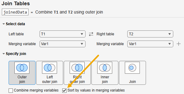
When joining tables using the Join
Tables Live Editor task, you can specify the ordering of output table
rows by using the Sort by values in merging variables check box.
Previously, Join Tables always sorted output table rows by
values in the merging variables. To return the output table without sorting the rows, clear
the Sort by values in merging variables check box. Clearing this check
box is equivalent to calling innerjoin or
outerjoin with the RowOrder="stable" name-value
argument.
Specify row order of output table for inner and outer joins
Create and work with datetime arrays in different time
standards
You can now create and work with datetime arrays in International Atomic Time (TAI) and Terrestrial Time
(TT), in addition to Coordinated Universal Time (UTC), by using the
TimeStandard name-value argument and property. These time standards
are useful in domains such as aerospace, astronomy, and telecommunications, where the
simplified version of UTC representation, which does not account for leap seconds, is
insufficient.
To specify a time standard, use the TimeStandard name-value argument
with the datetime function.
t = datetime("now",TimeStandard="TT");
To convert the time standard of an existing datetime array, set the
TimeStandard property to a new supported value.
t.TimeStandard = "TAI";CLDR upgraded to version 46 with updated locale data for datetime
arrays
The Common Locale Data Repository (CLDR) locale data is upgraded to version 46. The
datetime data type uses CLDR locale data for
localized names and locale-specific date and time formats. For more information, visit
cldr.unicode.org.
Preserve end-of-month and end-of-quarter dates in arithmetic with
calendarDuration values
In datetime arithmetic, calendarDuration values can now preserve end-of-month or end-of-quarter
dates by using the ArithmeticMethod name-value argument. To create
calendarDuration arrays that preserve month ends in arithmetic, use
calendarDuration with
ArithmeticMethod="endofmonth" or use calmonths. To create calendarDuration arrays that
preserve quarter ends in arithmetic, use calendarDuration with
ArithmeticMethod="endofquarter", or use calquarters.
If you load a calendarDuration array with the
ArithmeticMethod property into an earlier MATLAB release (R2014b
through R2026a), the earlier release ignores the ArithmeticMethod
property, and the loaded calendarDuration array uses the default
arithmetic method that preserves the day of the month when possible.
The caldiff and between functions now support datetime difference
computations with respect to month ends and quarter ends. The isregular function now supports end-of-month and end-of-quarter regularity
detection. Timetables with row times that occur at the end of each month or quarter can now
be treated as regular, so you can create and manipulate timetable data more easily.
Specify naming rule for variables in grouped summary table
When using the groupsummary
function with table or timetable input data, you can control how variables in the output
table are named. Specify the VariableNamingRule name-value argument as
"methodname" to use the names of the computation methods as prefixes
(for example, mean_Var1 or myFun_Var1), or as
"noprefix" to match the variable names in the input data (for
example, Var1).
Also, in the Compute by Group task,
when you specify a computation method as a function handle, the name of the corresponding
output table variable now includes a prefix derived from the function name (for example,
myFun_Var1). Previously, the prefix was a generic label with a number
(for example, fun1_Var1).
Explicitly control whether to normalize polynomial query points
Specify the Normalize argument to explicitly control whether the
polyfit function normalizes
the query points before fitting a polynomial to the input data.
If you specify Normalize=true, polyfit centers
the query points at 0 and scales them to a standard deviation of
1 before fitting. The returned polynomial coefficients and fit
statistics are expressed in terms of the normalized query points
Previously, normalization was controlled implicitly by the number of output arguments.
For example, specifying a third output argument, as in [coeffs,~,centerScale] =
polyfit(x,y,n), automatically normalized the query points. This syntax is
still supported. However, using Normalize is recommended because it
makes the normalization behavior explicit and independent of the number of output
arguments.
Return cross-correlation or cross-covariance for nonnegative or nonpositive lags
You can return the cross-correlation or cross-covariance for only nonnegative or
nonpositive lags by specifying the LagSelection argument with the
xcorr or
xcov
function. Specify LagSelection as "nonnegative" to
return values for lags from 0 to maxlag, or as
"nonpositive" for lags from -maxlag to
0.
Compute cross-correlation or cross-covariance using sparse inputs
categorical Data Type: Find elements by pattern matching using
matches, startsWith, endsWith,
and contains functions
The matches,
startsWith, endsWith, and contains functions now support categorical
arrays as the input array. Use these functions to determine whether elements in a
categorical array have category names that match, start with, end with, or contain a
specified pattern.
Run Experiment Manager experiment and access result programmatically
You can now run an experiment and access a result from an experiment without opening the Experiment Manager app by using these functions:
runExperiment— Run an experiment and return anExperimentResultobject. If you have Parallel Computing Toolbox™, you can specifyUseParallel="on"to run experiment trials simultaneously.experimentResult— Retrieve an existing result of an experiment as anExperimentResultobject.experimentTrial— Retrieve a trial from an existing result of an experiment as anExperimentTrialobject.experimentNames— List the names of experiments in a MATLAB project.experimentResultNames— List the names of existing results from an experiment.
You must create and configure your experiments using the Experiment Manager app.
Data Import and Export
Read and write data using Google Sheets
You can read and write data directly from Google
Sheets™ spreadsheets using existing functions, such as readtable, writetable, readmatrix,
writematrix,
readcell,
writecell,
readtimetable, writetimetable, and sheetnames. To access a Google
Sheets spreadsheet, specify the spreadsheet URL or spreadsheet ID as the filename
input.
For example, read a Google Sheets spreadsheet into a table.
url = "https://docs.google.com/spreadsheets/d/SPREADSHEET_ID";
T = readtable(url);
Write a MATLAB table to an existing Google Sheets spreadsheet.
T = table([1;2;3],["a";"b";"c"],VariableNames=["Row","Label"]);
writetable(T,url);
You can use the Sheet and Range name-value
arguments to specify a particular sheet or cell range within the spreadsheet.
T = readtable(url,Sheet="Sheet2",Range="A1:D10");
writetable(T,url,Sheet="Results",Range="A1");
Before you can access Google Sheets from MATLAB, you must connect your Google® account to MATLAB using the Connections panel. For more information, see Read and Write Data from Your Google Account.
Create and manage Amazon S3 connections using Connections panel
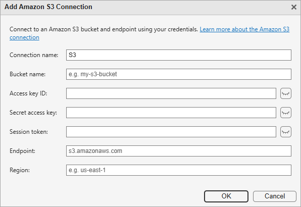
You can now create, configure, and manage multiple Amazon S3 connections directly from the Connections panel in MATLAB. Previously, accessing remote data in Amazon S3 required configuring credentials programmatically. Using the Connections panel, you can interactively set up connections by specifying a bucket name, Amazon Web Services (AWS) access key ID, and secret access key. Optionally, you also can specify the session token (if you are using temporary security credentials), the endpoint, and the geographic region of your bucket.
To create an Amazon S3 connection, go to the Home tab, and in the Environment section, click the Connections button to open the Connections panel. Then, in the Available Connections section, click the Add button next to Amazon S3.
For more information, see Work with Remote Data.
List file and folder names in natural order using dir
The dir function can now return folder contents
in natural order using the SortOrder name-value argument. Natural order
sorting treats numeric portions of filenames as numbers rather than characters. For
example, listing = dir("ExampleFolder",SortOrder="natural") lists
file2 before file10.
Specify S3 and Azure locations using https URLs
When you use MATLAB functions, such as readtable and writetable, to access remote data in Amazon S3™ and Azure® Blob Storage locations, you can now specify standard
https:// URLs, in addition to existing support for the
s3:// and wasbs:// schemes.
Resolve relative paths to absolute paths
The new resolveFilePath function returns the absolute paths of files and folders.
Use this function to convert relative paths or partial paths to fully qualified absolute
paths.
NetCDF functions support 64-bit data format
You can query, read, and write data from existing 64-bit data format (CDF-5) files using
the netCDF
functions. Create new 64-bit data format files using the netcdf.create function.
XSLT processor upgraded to Saxon 9b
The xslt function now uses the Saxon 9b XSLT
processor.
Validate file information using new validation functions
Use these new validation functions to validate file information:
mustBeFilePathInclusive— Validate that a value is a file in the current folder, at the specified location, or on the MATLAB path.mustBeSymbolicLink— Validate that a value is a symbolic link.
For more information about using validation functions for function argument and property checks, see Function Argument Validation and Property Validation Functions.
Functionality being removed or changed
web function opens local files in HTML Viewer when MATLAB started with -nodesktop option
Behavior change
When you start MATLAB with the -nodesktop option and use the web function to open a local URL or file, the page now opens in the HTML
Viewer. Previously, the page opened in a web browser.
xmlread function uses MAXP as the default XML processing
engine
Behavior change
The xmlread function now uses the MATLAB API
for XML Processing (MAXP) as the default XML processing engine. Previously, the
xmlread function used the Java API for XML Processing (JAXP) by default. To specify JAXP, set the
XMLEngine name-value argument to "jaxp".
serial function now errors
Errors
serial and its object properties now error and will be removed in
a future release. Use serialport
and its properties instead.
This example shows how to connect to a serial port device using the recommended functionality.
| Functionality | Use This Instead |
|---|---|
s = serial("COM1");
s.BaudRate = 115200;
fopen(s) |
s = serialport("COM1",115200); |
For more information about updating your code to use the recommended functionality, see Transition Your Code to serialport Interface.
Mathematics
Generate random numbers using two new algorithms: "pcg" and
"xoshiro"
You can use two new algorithms for random number generation.
| Name | Algorithm | Multiple Stream and Substream Support | Description | Approximate Period in Full Precision |
|---|---|---|---|---|
"pcg" |
| Yes | 64-bit permuted congruential generator with double xor-shift multiply | 2255 (263 streams of length 2192) |
"xoshiro" |
| Yes | Xor-shift-rotate generator with 256-bit state and double addition | 2256 (264 streams of length 2192) |
Both algorithms also provide the option to use full precision, and they use
"Inversion" as the default normal transform.
To select these generator algorithms when controlling the MATLAB random number generator using the rng function, specify the generator name, such as
rng("pcg") or rng("xoshiro"). You can also set
either generator as the default by specifying it in the MATLAB Settings Window.
To select these generator algorithms when creating and controlling a random number
stream using RandStream or RandStream.create, specify either the generator algorithm or its name, such
as RandStream("pcg64dxsm") or
RandStream("pcg").
Additional support for RandStream object
The RandStream object has several improvements:
You can now create a copy of an existing random number stream with the same properties and state using the syntax
s =
                     RandStream(existingStream)
. When you generate random numbers using the newly copied stream and the existing stream, sampling from one stream does not affect the other.When creating a
RandStreamobject, you can choose whether to generate antithetic random numbers or whether to use full precision by specifying theAntitheticorFullPrecisionname-value argument, respectively.When using
RandStream.list, you can now specify an output argument to return a table of all available generator algorithms. The table provides detailed information for each algorithm, including the generator name, multiple-stream support, and description.
The RandStream object also has some changes in behavior:
For a random number stream that uses
"Polar"as the normal transformation algorithm, saving and restoring the internal state of the stream now accurately reproduces the sequence of random numbers.For example, create a random number stream using the Mersenne Twister algorithm and the polar normal transformation. Generate a random number from this stream, and save the stream state before generating a second random number.
s = RandStream("twister",NormalTransform="Polar");
n1 = randn(s);
savedState = s.State;
n2 = randn(s)
Next, restore the stream state to the previously saved state. Generate a third random number. The second and third random numbers are the same.n2 = -0.7733
s.State = savedState;
n3 = randn(s)
In previous releases, this code produced different values for the second and third random numbers.n3 = -0.7733
Calling
RandStream.listwithout an output argument now displays a table of all available generator algorithms with more detailed information about the generators, including their names and multi-stream support. In previous releases,RandStream.listdisplayed only the available generator algorithms and their descriptions.
Evaluate definite integral with variable upper limit
You can evaluate a definite integral with a variable upper limit using the new integralInterpolant object. You can also calculate the interpolated integral
at values in the interval by querying the integralInterpolant object at a
point or set of points.
Specify points of interest in integration region
Additional support for ordinary differential equations
The ode object and
ODEResults
object have new properties that you can use when solving ordinary differential equations:
You can specify the exact time values that you want the ODE solver to reach by setting the
Waypointsproperty of theodeobject. The solver reaches the specified time values by adjusting its step size.You can calculate the Jacobian of a complex equation using automatic differentiation by setting the
JacobianMethodproperty of theodeobject to"autodiff".You can identify why the integration of an
odeobject stopped by using the newStopReasonproperty returned by theODEResultsobject. TheStopReasonproperty indicates if the solver completed the integration, stopped the integration due to a specified function or event, or failed to meet specified tolerances during integration.You can set a lower bound on the step size of any step taken by SUNDIALS ODE solvers by setting the
MinStepproperty ofmatlab.ode.options.IDAS,matlab.ode.options.CVODESNonstiff, andmatlab.ode.options.CVODESStiffobjects, through theSolverOptionsproperty of theodeobject.
Graphics
Plot multiple data sets simultaneously with histogram,
binscatter, geoplot, and other functions
Now you can use more plotting functions to visualize multiple data sets simultaneously:
The
histogram,polarhistogram, andstem3functions support plotting multiple table variables.The
binscatter,geoplot,geodensityplot, andgeoscatterfunctions support plotting multiple table variables and matrices of coordinates.
To accommodate multiple data sets, binscatter plots now support
transparency. When you create multiple binned scatter plots, each distribution has a
different overall hue by default, and transparency varies across the tiles according to the
bin counts. If you plot one binned scatter plot, the plot is opaque and has the same
appearance as in previous releases.

Export figures as web canvases interactively
Create HTML files that contain interactive web canvases by selecting Save As > Export To in the figure toolstrip or by using the uiexportdlg
function. In both approaches, select the HTML format option in the Export dialog box to
export a figure as a web canvas.

For more information, see Print or Export Figure from Figure Toolstrip.
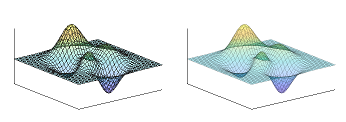
Configure semitransparent edges and meshes of function plots
Control the transparency level of the edges and meshes of function plots created with
the fsurf, fmesh, and fimplicit3 functions by setting the
EdgeAlpha property of the plot to a number between 0 and
1. A value of 0 makes the edges completely
transparent and 1 makes the edges opaque.
Maximize geographic axes by filling available space
Maximize geographic axes by filling the available space within the parent container. To
maximize the axes, set the MapLayout property of the GeographicAxes object to
"maximized". Maximizing the axes hides the axis labels, ticks, tick
labels, grid, and titles. The default for MapLayout is
"normal", which displays the axes in a box that is inset from the
edges of the parent container.
This image compares the normal map layout and the maximized map layout.

Display or hide axes toolbar in stacked plots and geographic bubble charts
Display or hide the axes toolbar in charts created with the stackedplot
and geobubble functions by setting the
ToolbarVisible"off".
Functionality being removed or changed
GraphicsSmoothing and FontSmoothing properties
will be removed
Warns
MATLAB issues a warning if you set or get the value of the
GraphicsSmoothing property of a figure or the
FontSmoothing property of axes, rulers, and text objects. These
properties will be removed in a future release. Since R2025a, all graphics and text are
smooth regardless of the value of these properties.
MATLAB issues an error if you set or get the FontSmoothing
property of a GeographicScalebar object.
plotyy will be removed
Still runs
The plotyyyyaxis function instead.
The yyaxis function has several advantages over the
plotyy function.
Unlike
plotyy, theyyaxisfunction creates oneAxesobject with two y-axes.plotyycreates two overlaidAxesobjects that can get out of sync.You can use
yyaxiswith any 2-D plotting function, including functions with varied syntaxes, such aserrorbar. By contrast,plotyyis limited to working with plotting functions of the formfunction(x,y).
This table shows some typical uses of plotyy and how to update
your code.
| Not Recommended | Recommended |
|---|---|
plotyy(x1,y1,x2,y2) |
yyaxis left plot(x1,y1) yyaxis right plot(x2,y2) |
plotyy(x1,y1,x2,y2,'function1','function2') |
yyaxis left function1(x1,y1) yyaxis right function2(x2,y2) |
App Building
Save App Designer apps in plain text file format to use with source control
You can save App Designer apps in a new plain text file format, which is useful for
source control integration. The plain text app format consists of two files: an app code
file (.m) and an app configuration file (.xml). Both
files can be opened in App Designer and in other editors. For more information, see App Designer File Formats.
Add UI components to app canvas using quick insert menu
In App Designer Design View, you can add UI components to an app by double-clicking the app canvas and selecting a component from the quick insert menu. For more information, see Lay Out Apps in App Designer Design View.
Interactions with Code Browser and Property Inspector in App Designer have new keyboard shortcuts
In App Designer, you can now interact with the Code Browser and Property Inspector using new keyboard shortcuts. To move focus between tab headers, use the left and right arrow keys. When the intended tab is in focus, use the Tab key to navigate through the content.
In previous releases, there were no keyboard shortcuts to move focus between tab headers or navigate through content in the Code Browser or Property Inspector.
For more information, see App Designer Keyboard Shortcuts.
Manage layout and exclusive selection of radio buttons or toggle buttons
For improved layout control, you can now parent radio buttons (created using uiradiobutton) and toggle buttons (created using uitogglebutton) directly to figures, tabs, panels, and grid layouts.
Previously, radio buttons and toggle buttons had to be parented to button groups.
To manage the exclusive selection of a set of radio buttons or toggle buttons, create a
selection group using the new uiselectiongroup function. For more information about selection groups, see
SingleSelectionGroup.
If you do not specify a parent container when creating a radio button or a toggle
button, MATLAB now calls the uifigure function to create a new
Figure object that serves as the parent container. Previously,
uibuttongroup created the default parent container.
The default Position property value for radio buttons (created
using uiradiobutton) is now [100 100 91 22].
Previously, the default value was [10 10 91 22].
The default Position property value for toggle buttons (created
using uitogglebutton) is now [100 100 100 22].
Previously, the default value was [10 10 100 22].
Test apps using the new double-press gesture and updated existing gestures
The app testing framework introduces the double-press gesture and extends support for existing gestures:
Perform double-press gestures on list box items using the new
doublePressmethod. For an example, see Double-Press List Box Items.Perform press gestures on button groups using the
pressmethod. For an example, see Press Button Group.Perform press gestures on axes toolbar buttons using the
pressmethod. For an example, see Press Axes Toolbar Buttons.Perform drag gestures on map axes (requires Mapping Toolbox™) using the
dragmethod. For an example, see Drag Between Points on Map Axes.
Functionality being removed or changed
Figures that have a menu bar or a toolbar no longer support desktop docking
Behavior change
CurrentObject property of Figure updates on
clicks and key presses
Behavior change
For a Figure object, MATLAB now sets the CurrentObject property to the last object selected in the figure, in
response to both clicks and key presses. Previously, the
CurrentObject property updated in response to clicks
only.
Performance
datetime Data Type: Improved performance with
datetime arrays
Operations on datetime
Array creation
Array indexing
Reshaping
Converting different data types to
datetime
For example, this code creates a datetime scalar. The code is about 11x
faster than in the previous release.
function timingTest
for i = 1:1e5
    d = datetime(2026,1,1);
end
end
The approximate execution times are:
R2026a: 2.22 s
R2026b: 0.19 s
As another example, this code gets the size of a datetime vector. The
code is about 43x faster than in the previous release.
function timingTest
d = [datetime("yesterday") datetime("today") datetime("tomorrow")];
for i = 1:1e5
    s = size(d);
end
end
The approximate execution times are:
R2026a: 0.32 s
R2026b: 0.0073 s
The code was timed on a Windows 11, AMD EPYC™ 74F3 24-Core Processor @ 3.19 GHz test system using the timeit
function.
timeit(@timingTest)
groupsummary Function: Improved performance with string grouping
vector
The groupsummary
function shows improved performance when the input data is a large, numeric variable or
vector, the grouping variable or vector type is string, and you specify
at least one of the "sum", "mean",
"min", "max", "range",
"nummissing", or "nnz" computation methods.
For example, this code computes the minimum, mean, and maximum for a 5,000,000-element
numeric vector using a grouping vector of type string. The code is about
3.3x faster than in the previous release.
function t = timingTest
n = 5e6;
numGroups = 1e4;
A = rand(n,1);
groups = repmat(string(rand(numGroups,1)),n/numGroups,1);
G = @() groupsummary(A,groups,["min","mean","max"]);
t = timeit(G);
end
The approximate execution times are:
R2026a: 0.86 s
R2026b: 0.26 s
The code was timed on a Windows 11, AMD EPYC 74F3 24-Core Processor @ 3.19 GHz test system by calling the
timingTest function.
innerjoin and outerjoin Functions: Improved
performance for tall tables without sorting output rows
The innerjoin and outerjoin functions show improved performance when you join a tall table
with an in-memory table without sorting the rows of the output table. For information on
sorting, see the release note Specify row order of output table for inner and outer joins.
For example, these code blocks each perform an inner join of a tall table and an
in-memory table and gather the joined table into memory. The R2026b code calls
innerjoin with RowOrder="stable", which returns
the output table without sorting the rows. For workflows that do not require sorted output,
this approach is about 6.6x faster than the default sorted join behavior in R2026a.
| R2026a | R2026b |
|---|---|
function t = timeInnerJoinWithTall % Run tall code on the local MATLAB session mapreducer(0); % Create tall table x = randi(1e3,1e4,1); y = randi(1e3,1e4,1); t = table((1:length(x))',x,y,VariableNames=["keys","Var1","Var2"]); tallTable = tall(t); % Create in-memory table inMemoryTable = table(randperm(1e4,100)',x(1:100),y(1:100), ... VariableNames=["keys","Var3","Var4"]); % Measure time for innerjoin function timeInnerJoin C = innerjoin(tallTable,inMemoryTable); gather(C); end t = timeit(@timeInnerJoin); end |
function t = timeStableInnerJoinWithTall % Run tall code on the local MATLAB session mapreducer(0); % Create tall table x = randi(1e3,1e4,1); y = randi(1e3,1e4,1); t = table((1:length(x))',x,y,VariableNames=["keys","Var1","Var2"]); tallTable = tall(t); % Create in-memory table inMemoryTable = table(randperm(1e4,100)',x(1:100),y(1:100), ... VariableNames=["keys","Var3","Var4"]); % Measure time for innerjoin function timeInnerJoin C = innerjoin(tallTable,inMemoryTable,RowOrder="stable"); gather(C); end t = timeit(@timeInnerJoin); end |
The approximate execution times are:
R2026a: 0.53 s
R2026b: 0.08 s
The code was timed on a Windows 11, AMD®
EPYC 9474F 24-Core Processor @ 3.6 GHz with 64 GB RAM test system by calling the
timeInnerJoinWithTall and
timeStableInnerJoinWithTall functions.
jsondecode Function: Improved performance when decoding
JSON-formatted arrays
The jsondecode function shows improved
performance when decoding JSON-formatted arrays containing mixed numeric and text data. For
example, this code creates a JSON-encoded cell array where elements alternate between
numeric and text data, and then decodes it. The call to jsondecode is
about 1.2x faster than in the previous release.
function t = jsondecodePerformance
N = 1000*1000;
c = num2cell(randi([1 9],N,1));
c(2:2:end) = cellstr(string([c{2:2:end}]));
json = jsonencode(c);

f = @()jsondecode(json);
t = timeit(f);
end
The approximate execution times are:
R2026a: 0.36 s
R2026b: 0.30 s
The performance improvement is particularly noticeable for arrays of numeric data. For
example, this code creates a JSON-encoded array of one million random integers and decodes
it. The call to jsondecode is about 6x faster than in the previous
release.
function t = jsondecodePerformanceIntegers
N = 1000*1000;
json = jsonencode(randi([1 9], N, 1));

f = @()jsondecode(json);
t = timeit(f);
end
The approximate execution times are:
R2026a: 0.54 s
R2026b: 0.09 s
The code was timed on a Windows 11, AMD EPYC 74F3 24-Core Processor @ 3.19 GHz test system by calling the
jsondecodePerformance and
jsondecodePerformanceIntegers functions.
dir Function: Improved performance when recursive listing of
remote locations
The dir function shows improved performance
when recursively listing the contents of remote storage locations, such as Amazon S3 buckets. For example, this code recursively lists all files in a remote
Amazon S3 folder containing approximately 500 files and folders. The code is about 450x
faster than in the previous release.
function t = timingTest
dir("s3://example_bucket/example_folder/**/*");
end
The approximate execution times are:
R2026a: 1045 s
R2026b: 2.3 s
The code was timed on a Windows 11, AMD EPYC 74F3 24-Core Processor @ 3.19 GHz test system using the timeit
function. Execution times for remote operations also depend on network bandwidth, server
load, and the number of files in the remote location.
timeit(@timingTest)
ismember Function: Improved performance with string query and set
arrays
The ismember function shows improved
performance when both the query and set arrays are of type string. The
improvement is most noticeable when some elements of the query array are found in the set
array.
For example, this code determines which strings in a 100-element string array are also in a 3,000,000-element string array. The code is about 3.9x faster than in the previous release.
function t = timingTest
A = string(rand(100,1));
B = repmat(string(rand(1e3,1)),3e3,1);
Lia = @() ismember(A,B);
t = timeit(Lia);
end
The approximate execution times are:
R2026a: 0.59 s
R2026b: 0.15 s
The code was timed on a Windows 11, AMD EPYC 74F3 24-Core Processor @ 3.19 GHz test system by calling the
timingTest function.
islocalmin and islocalmax Functions: Improved
performance
The islocalmin
and islocalmax
functions show improved performance. The improvement is most noticeable when you do not
specify name-value arguments and you return only one output.
For example, this code finds the local maxima in a 50,000,000-element numeric vector. The code is about 3.4x faster than in the previous release.
function t = timingTest
A = rand(5e7,1);
f = @() islocalmax(A);
t = timeit(f);
end
The approximate execution times are:
R2026a: 1.00 s
R2026b: 0.29 s
The code was timed on a Windows 11, AMD EPYC 74F3 24-Core Processor @ 3.19 GHz test system by calling the
timingTest function.
unique Function: Improved performance with string input
data
The unique function shows improved performance
when the input data type is string. For example, this code finds the
unique values in a 2,000,000-element string array. The code is about 1.4x faster than in
the previous release.
function t = timingTest
A = repmat(string(rand(1e3,1)),2e3,1);
C = @() unique(A);
t = timeit(C);
end
The approximate execution times are:
R2026a: 0.40 s
R2026b: 0.29 s
The code was timed on a Windows 11, AMD EPYC 74F3 24-Core Processor @ 3.19 GHz test system by calling the
timingTest function.
polyshape Objects: Improved performance for Boolean operations with
a single input
The union and
intersect
functions show improved performance when called with a single input, such as
union(gv) and intersect(gv), where
gv is a vector of polyshape
objects.
For example, this code finds the union of 1000 polyshape objects. The
call to union is about 94x faster than in R2025b.
function t = timingTest
basePoly = polyshape([0 1 0.5],[0 0 1]);
P = repmat(polyshape,1000,1);
rng(42);
for k = 1:1000
    P(k) = translate(basePoly,[50*rand,50*rand]);
end
Q = @() union(P);
t = timeit(Q);
end
The approximate execution times are:
R2025b: 1.316 s
R2026b: 0.014 s
The code was timed on a Windows 11, Intel Core® i9-14900K @ 3.20 GHz test system with 128 GB memory by calling the
timingTest function.
nufftn Function: Improved performance for uniform-to-nonuniform
transformations
The nufftn
function shows improved performance when transforming data from uniformly spaced sample
points to nonuniformly spaced query points.
For example, this code creates a 1,000,000-by-3 matrix of nonuniform query points
F. The code then calculates the 3-D nonuniform discrete Fourier
transform along each dimension of a 100-by-100-by-100 array X,
transforming the data from the default uniform sample points to the nonuniform query
points. The code is about 1.6x faster than in the previous release.
function t = timingQueryPoints
n = 100;
F = rand(n^3,3);
X = rand(n,n,n);

Y = @() nufftn(X,[],F);
t = timeit(Y);
end
The approximate execution times are:
R2026a: 1.00 s
R2026b: 0.64 s
The code was timed on a Windows 11, AMD EPYC 74F3 24-Core Processor @ 3.19 GHz test system by calling the
timingQueryPoints function.
Create Plot Task: Improved performance when opening for the first time
The Create
Plot task shows improved performance when opening for the first time in
a MATLAB session. The delay between clicking Create Plot
and the task being ready is reduced. Because the Create Plot task
loads visualizations from your installed MathWorks® toolboxes and products, the improvement is most noticeable when many
toolboxes and products are installed.
For example, for a set of installed toolboxes and products that loads 91 visualizations, you can use the task about 1.9x sooner than in the previous release.
The approximate rendering times are:
R2026a: 30 s
R2026b: 16 s
The action was timed on a Windows 11, AMD EPYC 74F3 24-Core Processor @ 3.19 GHz test system by inserting the Create Plot task into a live script.
uislider Function: Improved performance when resizing an app with
multiple sliders in a grid
When you resize an app figure window that contains multiple sliders created using the
uislider function and those sliders are in
a grid layout manager, the app repositions its content faster in R2026b than R2026a.
For example, this code creates an app that contains 10 sliders in a grid layout manager and resizes the figure window. The code is about 1.5x faster than in the previous release.
function timingTest
f = uifigure;
g = uigridlayout(f,[5 2]);

for k = 1:10
    uislider(g);
end

widths = linspace(500,900,25);
heights = linspace(600,1000,25);
sizes = [widths(:),heights(:)];

for k = 1:size(sizes,1)
    f.Position(3:4) = sizes(k,:);
    drawnow;
end

close(f)
end
The approximate execution times are:
R2026a: 3 s
R2026b: 2 s
The code was timed on a Windows 11, AMD EPYC 74F3 24-Core Processor @ 3.19 GHz test system using the
timeit function.
timeit(@timingTest)
plot and plot3 Functions: Improved responsiveness
for large data visualizations
The plotplot3
For example, on a Windows 11, AMD EPYC 74F3 24-Core Processor @ 3.19 GHz test system that has 65 GB of system memory and an NVIDIA A16-2B GPU with 2 GB RAM, this code begins drawing content in the figure approximately 1.4x faster than in the previous release.
rng(11);
numLines = 12;
dataSize = 5e7;
x = linspace(0,10,dataSize);
y = sin(x + linspace(0,pi,numLines)') ...
       +0.01*cumsum(randn(numLines,numel(x)),2);
figure
plot(x,y)
This video compares the delay between executing the plot command and
the appearance of the plot in different releases. The left figure shows the R2026a
behavior, and the right figure shows the R2026b behavior.
Improved stability and memory usage for batch processing figures
When you create multiple figure windows using batch mode, parallel workers (requires Parallel Computing Toolbox), or in a standalone executable, the figure windows now consume less memory than in previous releases. To further reduce memory usage, close any figures that you no longer need.
Continuous integration and continuous delivery (CI/CD) workflows that open and close large numbers of figures have improved stability and memory usage. As a result, you can run automated processes that involve opening and closing large numbers of figures for a much longer period of time.
Heterogeneous Class Hierarchies: Improved performance for method invocation
Invoking methods defined in heterogeneous class hierarchies shows improved performance.
For example, the runMethodLoop function invokes the
getValue method on hCircle and hSquare
objects 1,000,000 times, and the loop is timed by the
methodHeterogeneous function. The code is about 600x faster than in
the previous release. (The full code for the heterogeneous hierarchy is listed at the end
of this note.)
function runMethodLoop(obj)
    for j = 1:1e6
        out = obj.getValue();
    end
end
function methodHeterogeneous
    obj = [hCircle,hSquare];
    f = @() runMethodLoop(obj);
    t = timeit(f)
end
The approximate execution times are:
R2026a: 7.6 s
R2026b: 0.012 s
The code was timed on a Windows 11, Intel® Xeon® CPU W-2133 6-Core Processor @ 3.60 GHz test system.
The root class of the heterogeneous hierarchy is hShape, and
hCircle and hSquare are subclasses. hCircle
and hSquare both inherit the getValue method from
hShape.
classdef hShape < matlab.mixin.Heterogeneous
    properties
        id = 1;
    end

    methods (Sealed)
        function out = getValue(obj)
            out = 3;
        end
    end
end
classdef hCircle < hShape
end
classdef hSquare < hShape
end
Heterogeneous Class Hierarchies: Improved performance for property access
Accessing properties defined in heterogeneous class hierarchies shows improved
performance. For example, the runPropertyLoop function reads the value
of property id in hCircle and hSquare
objects 1,000,000 times, and the loop is timed by the
propertyHeterogeneous function. To minimize overhead,
runPropertyLoop accesses the properties by passing them as
arguments to the function foo, which performs no operations on the
values. The code is about 20x faster than in the previous release. (The full code for the
heterogeneous hierarchy is listed at the end of this note.)
function runPropertyLoop(obj)
    for j = 1:1e6
        foo(obj.id)
    end
end
function propertyHeterogeneous
    obj = [hCircle,hSquare];
    f = @() runPropertyLoop(obj);
    t = timeit(f)
end
The approximate execution times are:
R2026a: 5.1 s
R2026b: 0.21 s
The code was timed on a Windows 11, Intel Xeon CPU W-2133 6-Core Processor @ 3.60 GHz test system.
The root class of the heterogeneous hierarchy is hShape, and
hCircle and hSquare are subclasses. hCircle
and hSquare both inherit the id property from
hShape.
classdef hShape < matlab.mixin.Heterogeneous
    properties
        id = 1;
    end

    methods (Sealed)
        function out = getValue(obj)
            out = 3;
        end
    end
end
classdef hCircle < hShape
end
classdef hSquare < hShape
end
function foo(varargin)
end
validatestring Function: Improved performance
The validatestring
function t = timingValidatestring
s = "omit";
opts = ["omitnan" "includenan"];

f = @() validatestring(s,opts);
t = timeit(f);
end
The approximate execution times are:
R2026a: 0.000150 s
R2026b: 0.000026 s
The code was timed on a Windows 11, AMD EPYC 74F3 24-Core Processor @ 3.19 GHz test system by calling the
timingValidatestring function.
MATLAB Build Tool: Improved performance when plotting and running tasks
Plotting and running tasks in a build file show improved performance due to faster task dependency analysis by the build tool. In general, the improvements become more noticeable as the number of tasks and dependencies in the build file increases. The greatest improvements occur in build files with dependent task groups that contain a large number of tasks.
For example, suppose you have a build file with two task groups named
"g1" and "g2", each containing 100 tasks, where
the "g2" task group depends on the "g1" task
group.
function plan = buildfile
import matlab.buildtool.Task

plan = buildplan;

plan("g1:t"+(1:100)) = Task;

plan("g2:t"+(1:100)) = Task;
plan("g2").Dependencies = "g1";
end
Plotting the tasks in the build file is about 4.8x faster than in the previous release. The approximate execution times are:
R2026a: 2.9 s
R2026b: 0.6 s
Running the tasks in the build file is about 1.5x faster than in the previous release. The approximate execution times are:
R2026a: 8.0 s
R2026b: 5.2 s
Plotting and running the tasks were timed on a Windows 11, Intel
Xeon 6-Core Processor @ 3.60 GHz test system using the timeit
function.
| Plotting Tasks | Running Tasks |
|---|---|
timeit(@() plot(buildfile)) |
timeit(@() buildtool("g2","-verbosity",0)) |
MATLAB Editor: Improved scrolling on high-DPI displays
Scrolling in the MATLAB Editor is smoother on high-DPI displays. When you scroll using the scrollbar on Windows systems with display scaling above 100% or on macOS systems, line numbers and code content move together. In previous releases, line numbers might visibly lag behind the code while scrolling.
For example, on a Windows 11, Intel Xeon W-2133 6-Core Processor @ 3.60 GHz test system with 64 GB RAM, if you set display scaling to 150%, open any file in the Editor, and scroll using the scrollbar, the line numbers and code update together.
This video compares the lag between the line numbers and code content while scrolling in different releases. The left side shows the R2026a behavior, and the right side shows the R2026b behavior.
Software Development
Save projects in TOML format for easier review and editing
The new matlab.toml
definition file type allows you to define and manage your entire project configuration in a
single TOML file. This format is easier to review and merge under source control, and you
can edit it directly in the MATLAB Editor.
With a TOML-based project, you can:
Manage project configuration, package dependencies, and file labels in one place.
Declare dependencies on MATLAB packages with version constraints, and automatically install them from configured repositories when the project opens.
Associate labels with file patterns so that matching files are labeled automatically.
Validate the TOML file to identify issues such as invalid syntax, invalid data, or missing files.
Detect missing package dependencies when running project checks.
To set the TOML format as the definition file type when you create a project, on the
Home tab, in the Environment section, click
Settings. Select MATLAB > Project and, in the New Projects section, set
Project definition files to
matlab.toml.
To convert an existing project to TOML format, use one of these methods:
On the Project tab, in the Environment section, click Settings. Then, in the Advanced section, edit Definition file type by clicking Change and selecting
matlab.toml.Use the
matlab.project.convertDefinitionFilesfunction.
You can add package dependencies from the project settings, from the
Dependencies tab, or by editing the matlab.toml
file directly.
For more information, see:
Share and install packages through File Exchange
MathWorks File Exchange is now a package repository, and add-ons installed
from File Exchange are installed as packages. File Exchange is on the list of known
repositories by default. You can remove File Exchange from the known repository list using
mpmRemoveRepository and add it again using mpmAddRepository. To get the File Exchange URL known to MATLAB, use the matlab.mpm.FileExchange function.
Share and install packages with custom repositories using MATLAB package repository service
A MATLAB package repository service acts as an intermediary between the MATLAB Package Manager and your organization's artifact management system (such as JFrog Artifactory). Set up a custom repository by following the steps outlined here, Distribute Packages Using MATLAB Package Repository Service.
Check projects with greater scope and in the background
When you run project checks, you now have the option to run the checks for the top-level project as well as all its referenced projects. For more information, see Run Project Checks.
You can also run project checks in the background. If you enable this option, when an event that triggers a background check occurs, MATLAB queues this check and runs all queued checks after a specified delay. For more information, see Configure Global MATLAB Projects Settings.
Identify project tests at the folder level
You can now mark folders in your project as test folders. The MATLAB unit testing framework uses these test folders to quickly identify and run tests in the project. For more information, see Add Test Folders.
Move project files and match names with functions more easily
You can move files and folders within a project, into a project, or out of a project by
using the moveFile
function. The function also allows you to rename files and folders.
To match files and folders more efficiently, the findFiles, listRequiredFiles, and listImpactedFiles functions now
support glob patterns for specifying files. You can use these glob patterns:
*— Match any characters within a single folder (nonrecursive wildcard).**— Match files and folders recursively.!— Exclude matches when used as a negation prefix./— Match directories only when used as a trailing slash.
Specify project shortcut names and groups programmatically
You can programmatically define the names and groups of your project shortcuts by
specifying the Name and Group name-value
arguments of the addShortcut function.
Filter project list to see files under source control
In the Project panel, you can filter files under the project root folder to view only the files that are tracked by source control. For more information, see Manage Project Files.
Projects created in empty folders have src and
tests folders
When you create a new project in an empty folder, MATLAB now automatically adds the src and
tests folders to the project. MATLAB does not add these folders if you create a project using the matlab.project.createProject function.
When you create a new project in any folder, you can also choose to initialize a Git™ repository.
Manage GitHub and GitLab connections from MATLAB
You can manage GitHub® and GitLab® connections directly from the MATLAB Connections panel. From the Connections panel, you can:
Manage GitHub or GitLab authentication.
Use one authentication workflow for GitHub or GitLab operations, including clone, fetch, push, and share.
Use multiple GitHub or GitLab accounts and link them to specific repositories.
Store authentication tokens securely in the MATLAB vault.
For more information, see Connect to GitHub or GitLab from MATLAB.
View pull requests and merge requests in MATLAB and share links to them
Use the Pull Requests panel to view and work with GitHub pull requests and GitLab merge requests directly within MATLAB.
View GitHub pull requests and GitLab merge requests without leaving MATLAB.
Compare files that changed in a pull or merge request, including Simulink® models.
Check out pull or merge requests locally to review and test changes.
Generate a shareable link to open GitHub pull requests or GitLab merge requests directly in a locally installed version of MATLAB.
For more information, see View and Share Pull Requests in MATLAB.
You can also generate links to view individual files on GitHub or open them in MATLAB Online™. In the Files panel, right-click the file you want to share and select Share > GitHub link or Share > Open GitHub file in MATLAB Online.
Custom MATLAB toolboxes are now called packages
The MATLAB language feature known as a toolbox is now
a package, and the associated installation file
(.mltbx) is now a package file.
Packages are collections of code bundled for distribution. As of R2026b, the terminology is
updated in both the documentation and software.
Package installation is handled by MATLAB Package Manager, which provides robust dependency management. MATLAB Package Manager is backward compatible with toolboxes created before R2026b. These toolboxes are supported and installed as packages.
You can interactively build a package in two ways:
If your code is in a MATLAB project, convert the project to the new TOML format, which enables the project to depend on packages. Open the project, go to the Project tab, and in the Tools section, click Build Package. MATLAB creates a package task with the same name as your project and opens it in the document area of the desktop.
If your files are not already included in a project, go to the Home tab, and in the Environment section, select Add-Ons > Build Package. Click Browse to select the folder containing your package files and then click OK. MATLAB creates a new project containing your files and a package task for configuring your package. If the folder you select already contains a project, the existing project is used instead. Configure the project to use the recommended TOML format.
To support MATLAB Package Manager functionality, the matlab.addons.toolbox.ToolboxOptions object includes three new properties:
PackageName, PackageDependencies, and
Readme.
For more information, see Share and Distribute Software.
Updates to support for packages
Packages have several improvements. You can:
Add custom labels — To make your package more easily searchable in repositories, including File Exchange, you can add custom package labels by using the
Tagsproperties of thematlab.mpm.Packageandmatlab.addons.toolbox.ToolboxOptionsobjects.Update installed packages — To update one or more installed packages to the latest available version or to a specific version, use the new
mpmupdatefunction.View changes before installation — To verify changes before you install a package, you can call
mpminstallwith the newDryRunname-value argument to see a list of all packages and dependencies to be installed, without installing them. If you also specifyAllowVersionReplacement=true, then packages to be removed are displayed as well.Add BSD license — To generate a BSD (Berkeley Software Distribution) license when building a package file (
.mltbx), set theUseLicenseBSDproperty of thematlab.addons.toolbox.ToolboxOptionsobject. TheUseLicenseBSDproperty must be true for package files uploaded to File Exchange.
Packages include extensions.json file
Packages built interactively or using matlab.addons.toolbox.packageToolboxextensions.json file. This file is created during the build
process if one does not exist.
MATLAB populates the extensions.json file using matlab.addons.toolbox.ToolboxOptions properties. The
ToolboxImageFile property registers the package image. The
AppGalleryFiles property determines app files registered with the
apps gallery. The ToolboxGettingStartedGuide property registers the
Getting Started guide.
Package installation logged by system audit logger
Package installation events are now logged by the system audit logger. MATLAB records the following information for each installed package and dependency:
Package ID
Originating repository
Download URL
Download destination
Package digest, as returned by
digest
Audit logger behavior varies by operating system. On Windows, system audit logging must be enabled. Open a Windows PowerShell command prompt as an administrator and run these commands:
$source = "MathWorks"
$logName = "Application"
$eventSourceExists = [System.Diagnostics.EventLog]::SourceExists($source)

if (-not $eventSourceExists) {
    [System.Diagnostics.EventLog]::CreateEventSource($source, $logName)
    Write-Host "Event source $source created successfully."
} else {
    Write-Host "Event source $source already exists."
}
You can then specify the severity level to log by creating a new
REG_DWORD value in the event source
HKEY_LOCAL_MACHINE\SYSTEM\CurrentControlSet\Services\EventLog\Application\MathWorks.
Set the REG_DWORD value to 0 to disable logging,
1 to log only critical events, 4 to log
notice-level events, or 7 to log events at all severity levels.
On Linux and macOS systems, audit logging is on by default. You can disable audit
logging or set the logging level by creating a file named
/etc/mathworks/settings.json on Linux and
/Library/Preferences/SystemConfiguration/MathWorks/settings.json on
macOS with this code:
{
  "auditlogging": {
    "level": "all"
  }
}
Set the level property to "none" to disable
logging, "critical" to log only critical events, and
"all" to log all events.
Specify files and folders for Code Analyzer to ignore during analysis
Configure the Code Analyzer to ignore specific files and folders during analysis by
using the "ignoredFiles" property in a Code Analyzer configuration file.
For more information, see Customize Code Analyzer Checks Using Configuration File.
Improved data model for build plan elements
The new matlab.buildtool.PlanElement class defines the minimal shared identity for all
elements that you can add to a build plan, such as tasks and task groups. The matlab.buildtool.Task and matlab.buildtool.TaskGroup classes now derive from the
PlanElement class and inherit its Name and
Description properties.
The new data model results in these changes:
The
Tasksproperty of thematlab.buildtool.Planclass represents plan elements as aPlanElementvector. In previous releases, the property contains aTaskvector instead.The
TaskGroupclass is no longer a subclass of theTaskclass. Therefore,TaskGroupno longer includes the properties that are unique to theTaskclass, such asActions,Inputs, andOutputs.
Speed up builds with task output caching
You can use task output caching in your builds by specifying the new
-outputCache option with the buildtool
command. When an output cache is available, the build tool skips tasks that can reuse
outputs from earlier builds, improving build performance. For more information, see Cache Task Outputs.
Build package from TOML project by using built-in task class
You can build a package from a TOML project by using the matlab.buildtool.tasks.PackageTask class. A task created from the
PackageTask class automatically uses the configuration in the matlab.toml
project definition file. For an example, see Build Package from TOML Project.
Generate build reports in HTML format
You can generate an HTML build report by using the generateHTMLReport method of the matlab.buildtool.BuildResult
class or the -report option of the buildtool
command. The build report provides detailed information about the build, including the
build environment, build summary, and individual task results.
Run tests using external parameters in MATLAB builds
You can inject new data into parameterized tests by using the
ExternalParameters property or task argument of the matlab.buildtool.tasks.TestTask class. For an example, see Run Tests Using External Parameters.
Visually identify cyclic task dependencies in build task plots
You can visually identify cyclic task dependencies by using the plot method of
the matlab.buildtool.Plan class. After plotting your tasks as a dependency
graph, verify that the graph is acyclic. If the graph contains cycles, update your build
plan to remove the cyclic dependencies.
In previous releases, the method throws an error and does not create a task graph if the build plan contains cyclic dependencies.
Emit MATLAB build telemetry data
You can instrument your MATLAB builds with OpenTelemetry™ to emit traces and metrics to observability backends. For more information, see Emit MATLAB Build Telemetry Data with OpenTelemetry Integration.
Test code insertion options in the Editor are goal oriented
The code insertion options in the Test section on the Editor tab now align with test authoring goals rather than programming concepts such as methods and properties. You can use these improved options to add tests to your test class and to specify setup code for individual tests or for the entire test class. For more information, see Insert Test Code Using Editor.
Use Test Browser when running tests with runtests
function
You can now use the Test Browser app
when running tests with the runtests function. To run tests and display
results using the test browser, specify the UseTestBrowser name-value
argument of the function as true.
If you run tests interactively from the Run Tests section on the
MATLAB Toolstrip with the Use Test Browser option selected, the
testing framework displays the command it uses to run the tests, including the
UseTestBrowser name-value argument. For more information, see Run Tests in Editor.
Add source code to Test Browser for coverage reporting by dragging files and folders
You can add source code to the Test Browser app for coverage reporting by dragging source files and folders from the Files or Project panel into the Source pane. To access the Source pane, click the Open coverage settings button on the Test Browser toolbar, and then select Enable coverage reporting.
Run tests in parallel with additional control
You now have more control over when to use a parallel pool to run tests using the
runtests function. The
UseParallel name-value argument of the function now accepts new
"off", "auto", and "on" values.
Specify UseParallel as "auto" to automatically
use a parallel pool if one is available or as "on" to always use a
parallel pool.
Starting in R2026b, specifying the UseParallel name-value
argument as true or false is not recommended. For
more information, see Logical values for
UseParallel argument of runtests
function are not recommended.
Unit testing framework discovers tests in project test folders
The unit testing framework now discovers and runs tests in project test folders. In XML
projects that define tests using both test folders and the Test
classification label on files, the framework includes tests from both sources in the test
suite. In TOML projects, test folders are the only way to define tests. For more
information, see Identify and Run Tests in MATLAB Projects.
Create preformatted diagnostics for constraints in unit tests
You can create preformatted constraint diagnostics using the convenience methods of the
matlab.unittest.constraints.Constraint and matlab.unittest.constraints.BooleanConstraint classes:
To create preformatted diagnostics inside the
getDiagnosticFormethod, use thecreatePassingDiagnosticandcreateFailingDiagnosticconvenience methods of theConstraintclass.To create preformatted diagnostics inside the
getNegativeDiagnosticFormethod, use thecreateNegativePassingDiagnosticandcreateNegativeFailingDiagnosticconvenience methods of theBooleanConstraintclass.
The convenience methods automatically set the matlab.unittest.diagnostics.ConstraintDiagnostic object properties required to
display the diagnostic information. For an example, see Create Custom Boolean Constraint.
Create UI figure using built-in test fixture
You can use the new matlab.unittest.fixtures.UIFigureFixture class to construct fixtures for
creating a UI figure. For an example, see Create UI Figures for Testing.
Test apps using the new double-press gesture and updated existing gestures
The app testing framework now includes the double-press gesture and extends support for existing gestures:
Perform double-press gestures on list box items using the new
doublePressmethod. For an example, see Double-Press List Box Items.Perform press gestures on button groups using the
pressmethod. For an example, see Press Button Group.Perform press gestures on axes toolbar buttons using the
pressmethod. For an example, see Press Axes Toolbar Buttons.Perform drag gestures on map axes (requires Mapping Toolbox) using the
dragmethod. For an example, see Drag Between Points on Map Axes.
Functionality being removed or changed
Calling mpminstall with Force=true installs
specified packages and dependencies even if it breaks existing dependencies
Behavior change
If you call mpminstall
with Force=true, and if a dependency of the installed package
conflicts with an already installed package or dependency, then the newly installed
dependency overwrites the installed package or dependency even if it breaks an installed
package.
For example, if installed packageA depends on version
1.0.0 of packageB and you call
mpminstall with Force as
true on packageC, which depends on version
2.0.0 of packageB, then
mpminstall overwrites version 1.0.0 of
packageB with version 2.0.0 and breaks the
dependency of packageA.
In previous releases, mpminstall does not overwrite installed
packages or dependencies if it would break the dependency of another installed
package.
Package installation folder name is derived from PackageName
property
Behavior change
When you install a package file (.mltbx), MATLAB creates a new folder in the designated installation area for the contents
of the package. Starting in R2026b, MATLAB derives the name of this folder from the PackageName
property of the corresponding matlab.addons.toolbox.ToolboxOptions
In previous releases, MATLAB derived the name of this folder from the ToolboxName
property.
ToolboxVersion property of ToolboxOptions
object must adhere to semantic version syntax
Behavior change
The ToolboxVersion property of the matlab.addons.toolbox.ToolboxOptions object must adhere to semantic version
syntax. ToolboxVersion syntax follows the Semantic Versioning 2.0.0 format:
<major>.<minor>.<patch>,
where each version number must be a nonnegative integer, for example,
1.2.3. You can optionally specify a pre-release version by adding
-<pre-release version> to
the end of the version, for example, 1.2.3-alpha. Optionally specify
a build version by adding +<build
version>. Previously, the ToolboxVersion
property accepted any text value without checking its format.
Description and RequiredAddons properties of
ToolboxOptions object are no longer supported
Still runs
The Description and RequiredAddons properties
of the matlab.addons.toolbox.ToolboxOptions object are no longer supported.
Instead, use the Readme property to direct your package users to a
file containing information about your package. Use the
PackageDependencies property to define packages that your package
depends on.
Logical values for UseParallel argument of
runtests function are not recommended
Still runs
Starting in R2026b, for the runtests function, specifying the UseParallel
name-value argument as true or false is not
recommended. Use the "off", "auto", and
"on" values instead.
This table shows how to update your code depending on your goal.
| Goal | Not Recommended | Recommended |
|---|---|---|
| Run tests in serial. | runtests(UseParallel=false) | runtests(UseParallel="off") (default) |
| Run tests in parallel, or if a parallel pool is not available, run them in serial. | runtests(UseParallel=true) | runtests(UseParallel="auto") |
| Run tests in parallel and error if a parallel pool is not available. | N/A | runtests(UseParallel="on") |
There are no plans to remove support for the true and
false values.
Rerunning failed tests uses a default test runner if the original runner no longer exists
Still runs
When you rerun failed tests using the rerun link in the test summary, the testing framework uses a default test runner instead of the original runner if you ran tests using one of these options:
A nondefault test runner created with the
testrunnerfunction or one of the static methods of thematlab.unittest.TestRunnerclass and that test runner no longer existsThe
runmethod of thematlab.unittest.TestCaseclass
In previous releases, the framework reruns failed tests using the original test runner.
External Language Interfaces
Call Java from MATLAB: Install OpenJDK JRE Runtime
MATLAB no longer includes Java Runtime as part of its installation. For information about installing OpenJDK, see Configure Your System to Use Java.
MATLAB now supports OpenJDK 25 Java from https://adoptium.net/. For
supported version information, see MATLAB Interfaces to Other Languages.
Before R2026b, if you call jenv or
matlab_jenv with the Java
version argument set to "factory", MATLAB set the Java path to the version included with MATLAB. Starting in R2026b, MATLAB no longer includes Java as part of its installation, and the argument value
"factory" is the same as "system", which
represents the default Java version on your system. Likewise, the JavaEnvironment
Configuration property value "factory" is the
same as "system", which represents the default Java version on your system.
Call C++ from MATLAB: Programmatically publish MATLAB interface to C/C++ libraries
You can programmatically configure and publish MATLAB interfaces to C/C++ libraries by
using objects in the clibgen.api
namespace. Use this approach instead of editing library definition files when you want to
modify a library interface. By defining the interface in MATLAB code, you can reuse the same definition across platforms and build
environments, resulting in a more maintainable and repeatable published interface.
Call MATLAB from C++: Pass custom C++ structures to MATLAB functions
You can pass custom C++ structures directly to MATLAB functions from a C++ engine application. Previously, you had to manually
convert structure fields to matlab::data::StructArray objects. Instead,
pass pointers to your native C++ structures as arguments to matlab::engine::MATLABEngine::feval and receive structure pointers as
outputs.
To pass custom C++ structures directly to MATLAB, you must start MATLAB using IN_PROCESS mode. For more information, see Pass C++ Structures to MATLAB Functions.
REST Function Service: Call MATLAB functions remotely from Python using REST services and native Python data types
The Python® class matlab.rest_function_service.client.MWHttpClient creates an object for calling
MATLAB functions in a REST function service. Use this object in your Python client applications to pass inputs to MATLAB functions and receive outputs using native Python data types. For more information, see Call MATLAB Functions from Python Using REST.
Call Python from MATLAB: Install Python version 3.13 from Add-Ons panel
Use the MATLAB Support for Python 3.13 add-on to install a version of Python that is compatible with MATLAB R2026b. For details on installing this add-on, see Install and Configure Python for Use in MATLAB.
For a list of additional MATLAB releases that support Python 3.13, see Versions of Python Compatible with MATLAB Products by Release.
Call Python from MATLAB: Interrupt out-of-process execution using Ctrl+C
When calling Python from MATLAB in out-of-process execution mode, you can now press Ctrl+C to interrupt long-running or unresponsive Python code and terminate the process. For more details about out-of-process execution mode, see Out-of-Process Execution of Python Functionality.
Support for Python version 3.14
MATLAB now supports Python version 3.14, in addition to versions 3.10, 3.11, 3.12, and 3.13. For supported version information, see Versions of Python Compatible with MATLAB Products by Release.
For more information about changes to Python support, see Python version 3.9 is no longer supported.
Support for .NET 8 or higher
MATLAB supports .NET 8 or higher, in addition to existing support for the Microsoft® .NET Framework. For more information about changes to .NET support, see MATLAB Interfaces to Other Languages.
Support for Perl 5.42.2 and Perl 5.44.0 on Windows
As of R2026a (May 2026), the version of Perl included with MATLAB for Windows is updated to Perl 5.42.2. In addition, as of R2026b, the version of Perl included with MATLAB for Windows is updated to Perl 5.44.0.
If you use the perl command on Windows, see https://www.perl.org/ for
information about using this version of Perl.
Compiler support for Intel oneAPI 2026
MATLAB supports Intel oneAPI 2026 with Microsoft Visual Studio® 2026 for C and C++ compilers for building C and C++ interfaces, MEX files, and standalone MATLAB engine and MAT-file applications on Windows.
Functionality being removed or changed
Python version 3.9 is no longer supported
Errors
Support for Python version 3.9 is discontinued. For continued support for your applications, upgrade to a supported version of Python. For supported version information, see Versions of Python Compatible with MATLAB Products by Release.
matlab.wsdl.createWSDLClient and
matlab.wsdl.setWSDLToolPath have been removed
Errors
The matlab.wsdl.createWSDLClient and
matlab.wsdl.setWSDLToolPath functions
have been removed.
Use the MATLAB RESTful functions (webread and webwrite) or the MATLAB HTTP interface instead. For more information, see Call Web Services from MATLAB Using HTTP.
Hardware Support
Arduino Hardware: Support for Raspberry Pi Pico 2 and Pico 2 W boards
You can now use MATLAB Support Package for Arduino® Hardware in the installed version of MATLAB to communicate with the Raspberry Pi® Pico 2 boards over USB and the Pico 2 W boards over USB and Wi-Fi®. For more information, see Supported Boards.
Arduino Hardware: Support for ESP32-S3-DevKitC boards
You can now use MATLAB Support Package for Arduino Hardware in the installed version of MATLAB to communicate with ESP32-S3-DevKitC boards over USB, Bluetooth®, and Wi-Fi. For more information on how to configure ESP32 boards, see Set Up and Configure ESP32 Hardware.
You cannot use the support package to connect these boards with an Adafruit® Motor Shield V2, motor carrier, CAN interface, or serial devices. The
function playTone and the name-value argument
AnalogReferenceMode of the arduino object in external mode do not support these boards. For more
information, see Supported Boards.
Arduino Hardware: Install Arduino-compatible libraries more easily
You can now use the arduinoio.customLibrary.downloadLibrary function to install Arduino-compatible libraries by specifying the library name, a GitHub® repository
URL, or a local ZIP file. In each case, the function installs the library and returns the
full path to the installed library folder.
Arduino Hardware: Create custom library template using
arduinoio.customLibrary.createLibraryTemplate function
You can now use the arduinoio.customLibrary.createLibraryTemplate function to get started with
creating a custom library.
The function generates a folder containing MATLAB and C++ templates for defining a custom library and establishing communication with Arduino hardware. You can then modify the templates to implement your own custom functionalities.