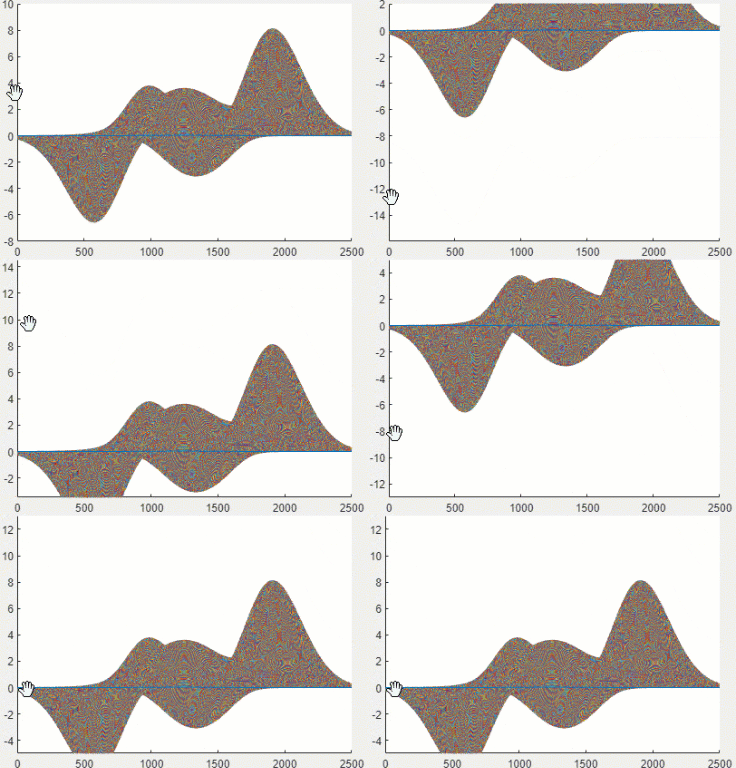
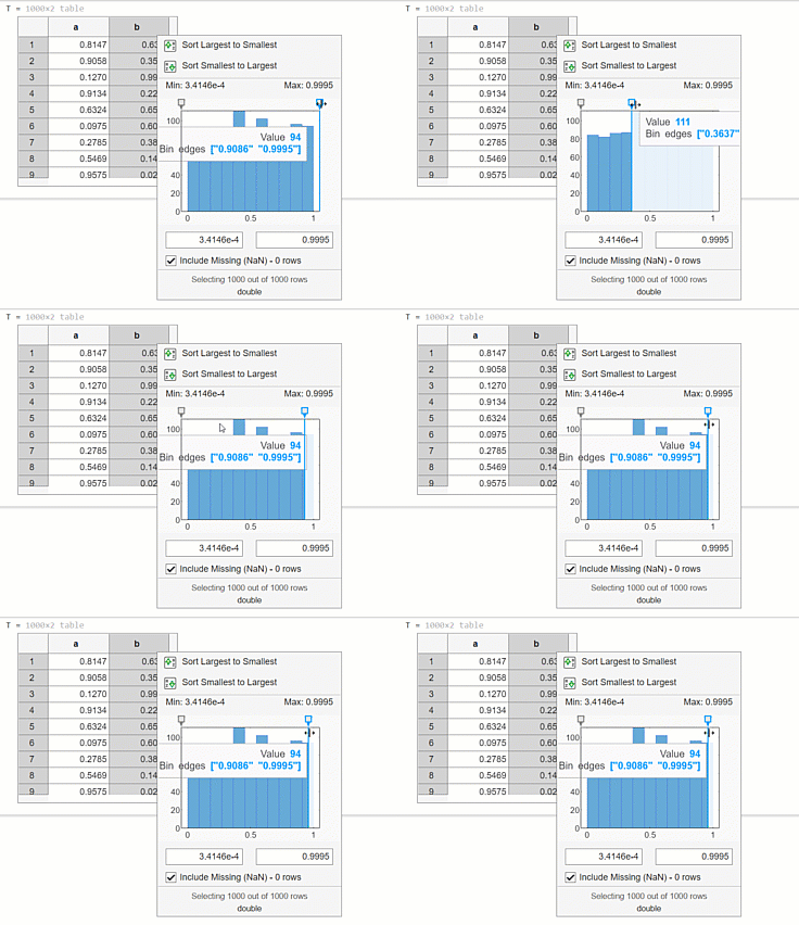
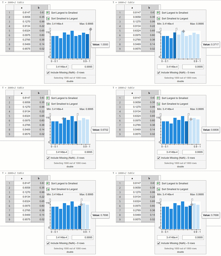
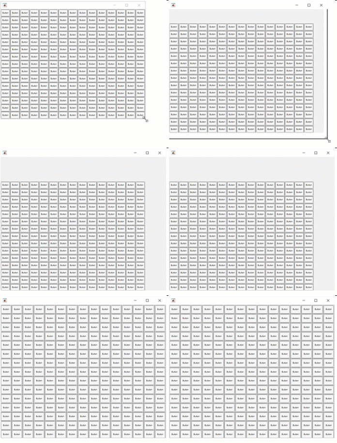
R2026b

New Features, Bug Fixes, Compatibility Considerations

Environment

   Java Runtime no longer installed with MATLAB

Before R2026b, MATLAB® installations on Windows® and Linux® platforms included Java® Runtime. Starting in R2026b, MATLAB no longer includes Java as part of its installation.

 Compatibility Considerations

You can download and install the MATLAB Support for OpenJDK® add-on or any compatible OpenJDK distribution after installing MATLAB. MATLAB continues to support OpenJDK on all platforms.

For information about supported versions, see Versions of OpenJDK Compatible with MATLAB by Release. MathWorks follows the vendors’ long-term support (LTS) guidance to determine versions for the MATLAB Support for OpenJDK add-on. Refer to the vendors’ websites for more information.

For information about changes to the jenv and matlab_jenv functions, see Call Java from MATLAB: Install OpenJDK JRE Runtime.

 Configure the desktop with more flexible layout options

You can configure the MATLAB desktop with greater layout flexibility.

  • Move more panels to the center of the desktop — Move the Files, Workspace, Command History, and Project panels to the center of the desktop.

  • Undock more panels — Undock the Debugger and Code Issues panels, allowing you to arrange them alongside an undocked Editor or Live Editor.

  • Reposition panels by dragging — Undock a panel or move it to the center of the desktop by dragging its title bar outside the MATLAB window or toward the center. For example, to move the Command History to the center of the desktop, drag the Command History panel title bar toward the center.

  • Identify and manage document groups using panel title bars — By default, documents in the center of the desktop include a title bar, which helps identify and manage document groups and panels. To show the title bar only when you hover over the edge of a document or panel tab, click the Panel actions button on the title bar and select Panel Headers > Show On Hover.

MATLAB also restores document locations more reliably in a session, preserving your desktop layout when you close and reopen documents.

For more information, see Configure the Desktop.
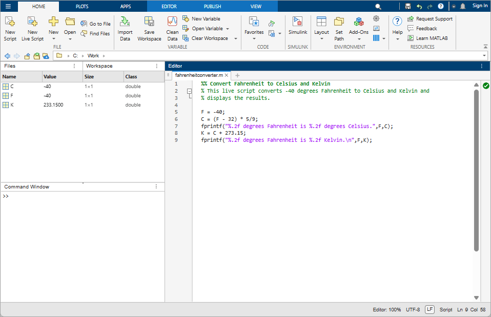
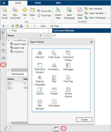
MATLAB desktop configured with a custom layout. The Files and Workspace panels are open and tiled on the left with the Command Window underneath them. The Editor is open in the middle of the desktop."

 Generate and display formatted text in the Command Window

You can render Markdown text and LaTeX equations directly in the Command Window and Live Editor using the markdowndisp function.

For example, you can display bold and italic text and an equation.
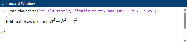
Command Window showing rendered bold text, italic text, and the equation a squared plus b squared equals c squared from markdowndisp

In addition, the Command Window now renders ANSI escape codes for styled and colored text, including bold, underlined, italic, and strikethrough formatting, as well as foreground and background colors. To display styled and colored text, use the fprintf, sprintf, or compose functions.

For example, you can display bold and blue text in the Command Window.
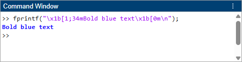
Command Window displaying bold blue text output from fprintf with ANSI escape codes

Large matrices are truncated in Command Window display

The Command Window now truncates most large two‑dimensional numeric matrices by default. To view the contents of a truncated matrix, click the link below the matrix. You also can view the contents by right-clicking the matrix or pressing Ctrl+D to open it in the Variables editor.

To disable truncating matrices by default, on the Home tab, in the Environment section, click Settings. Select MATLAB > Command Window, and in the Display section, clear the Show enhanced output (truncate matrix, render Markdown) option.
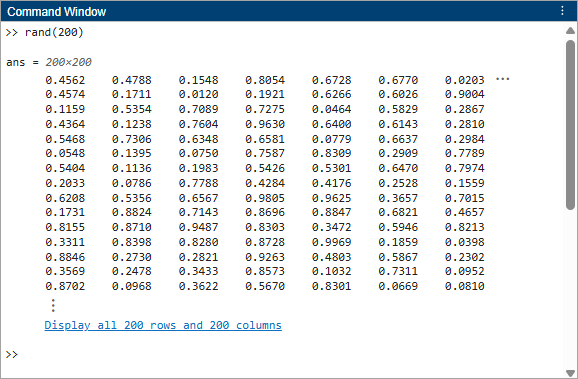
Command Window showing a truncated 200-by-200 matrix with a link to display all rows and columns

 Live scripts use plain text file format by default

By default, MATLAB creates and saves live scripts and live functions using the plain text live code file format (.m). This file format improves integration with source control and allows you to open live code files in external text editors. Live scripts saved in the plain text file format behave the same as other live scripts. They open in the Live Editor and can include code, output, formatted text, interactive controls, and tasks.

For more information, see Live Code File Formats.

Display long code lines using wrapping in the Editor

If your code file contains long code lines, the Editor or Live Editor can display those code lines across multiple visual lines without adding line breaks. This display-only wrapping helps you avoid horizontal scrolling while preserving the original code.

To enable wrapping long code lines, go to the View tab, and in the Display section, toggle the Wrap Code Lines button on. For more information, see Edit and Format Code.

Code file in the Editor showing a long expression on line 1 wrapped across two visual lines

Change end-of-line sequence for files open in the Editor

To change the end-of-line sequence for the file currently open in the Editor, click the end-of-line sequence indicator at the bottom-right corner of the MATLAB desktop and select the end-of-line sequence style to use.

For more information, see Change Line Endings.
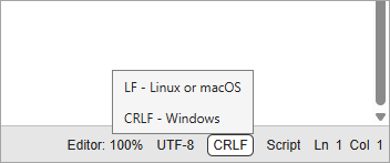
Bottom-right corner of the MATLAB desktop showing the end of line sequence indicator with the current value set to CRLF. The expanded menu displays two options: LF (for Linux or macOS) and CRLF (for Windows).

Add variable selector to live scripts

You can add a variable selector to your live script to select a workspace variable interactively. To add a variable selector, go to the Live Editor tab, and in the Code section, select Control > Variable Selector.
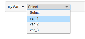
Variable selector expanded to show three variables, var_1, var_2, and var_3. The variable selector is assigned to the variable myVar.

For more information, see Add Interactive Controls to Live Scripts.

Go to specific line and column in the Editor using improved interface

Use the improved Go To interface to navigate to a specific location in a file open in the Editor or Live Editor more quickly. To navigate to a specific location, on the Editor or Live Editor tab, in the Navigate section, select Go To > Line. Then, specify the line and optionally the column number that you want to navigate to.

Go To interface with a text box to enter the line and column numbers

Examine file and folder comparison results directly at MATLAB Command Window

You can now use the visdiff function to examine folder and file comparison results directly at the Command Window. The comparison object now has a new Result property that contains information such as line-by-line comparison. For more information, see visdiff.

You can now close all currently opened comparison windows using the comparisons.closeAll command.

Register external text merge tool

By default, to resolve merge conflicts in text-based files, MATLAB uses a built-in two-way text merge tool. You can now use an external three-way merge tool for specific text file extensions, including .m, .txt, and .toml. For more information, see Register External Text Merge Tool.

 Functionality being removed or changed

Add-On Manager replaced by Add-Ons panel

Behavior change

The Add-On Manager has been removed. To find, install, and manage add-ons interactively, use the Add-Ons panel instead. For more information, see Get and Manage Add-Ons.

Add-on management using matlab.addons functions changed and replaced

Behavior change in future release

These matlab.addons functions are not recommended:

There are no plans to remove the matlab.addons functions. However, to manage add-ons, including enabling or disabling add-ons, a more efficient approach is to uninstall and reinstall add-ons using mpminstall and mpmuninstall, or to use MATLAB projects to manage add-on dependencies for your code. The mpmlist function provides additional support for listing installed add-ons.

This table shows some typical uses of the matlab.addons functions and how to update your code to use the mpminstall, mpmuninstall, and mpmlist functions instead.

Not RecommendedRecommended
installedAddon = matlab.addons.install("C:\Downloads\My toolbox.mltbx")installedAddon = mpminstall("C:\Downloads\My toolbox.mltbx")
installedAddon = matlab.addons.install("C:\Downloads\My toolbox.mltbx","overwrite")installedAddon = mpminstall("C:\Downloads\My toolbox.mltbx", AllowVersionReplacement=true)
installedAddon = matlab.addons.install("C:\Downloads\My toolbox.mltbx","add")installedAddon = mpminstall("C:\Downloads\My toolbox.mltbx", AllowVersionReplacement=false)
matlab.addons.uninstall("GUI Layout Toolbox") mpmuninstall("GUI Layout Toolbox")
installedToolbox = matlab.addons.toolbox.installToolbox("C:\Downloads\My toolbox.mltbx")installedToolbox = mpminstall("C:\Downloads\My toolbox.mltbx")
matlab.addons.toolbox.uninstallToolbox("GUI Layout Toolbox") mpmuninstall("GUI Layout Toolbox")
toolboxes = matlab.addons.toolbox.installedToolboxesaddons = mpmlist

As part of this change, you can no longer use the agreeToLicense argument with the matlab.addons.install and matlab.addons.toolbox.installToolbox functions to accept or review a license agreement before installing an add-on or toolbox. License agreement approval now occurs by default, and the license agreement and service level agreement (SLA) coverage remain in effect, even if the license is not displayed during installation.

To view the license agreement for an add-on, go to the Add-Ons panel, and in the Installed section, click the Options button to the right of the add-on. Then, select Open Folder to open the root folder of the add-on in the Files panel, where you can access the license agreement.

In addition, when you uninstall an add-on using the matlab.addons.uninstall or matlab.addons.toolbox.uninstallToolbox functions, the add-on is removed from the MATLAB path, but the add-on files are not removed from disk. Previously, the add-on files were removed from disk.

Language and Programming

Validation Functions: Validate that values are scalars, vectors, or empty arrays

Use the mustBeScalar validation function to validate that a value is a scalar. Use the mustBeVectorOrEmpty validation function to validate that a value is either a vector or an empty array. These functions extend the existing checks mustBeScalarOrEmpty and mustBeVector, providing more robust size checking in function argument and property validation.

For more information, see Function Argument Validation and Property Validation Functions.

Use screen reader and keyboard to navigate Debugger panel

You can use a screen reader and keyboard shortcuts to navigate and interact with the Debugger panel. Collapse and expand files using the left and right arrow keys, enable or disable breakpoints by pressing the space bar, navigate to breakpoints by pressing Enter, and remove breakpoints by pressing Delete.

For more information about the Debugger panel, see Manage Breakpoints in Debugger Panel.

Debug code using ValidHandle property for matlab.lang.WeakReference class

The new ValidHandle property in the matlab.lang.WeakReference class holds the same value as the Handle property, but if they hold a reference to an invalid handle object, MATLAB errors when you try to access ValidHandle. Use ValidHandle to help debug your code when breaking strong reference cycles.

Programmatically add subclasses and superclasses in Class Diagram Viewer addSubclasses and addSuperclasses methods

The new addSubclasses and addSuperclasses methods of matlab.diagram.ClassViewer add subclasses and superclasses, respectively, of the specified class to the Class Browser and canvas of a Class Diagram Viewer instance.

Warn when older class name is used after creation of new alias

WarnOnOldName is an optional name-value argument for the addAlias method of matlab.alias.AliasFileManager. When you set WarnOnOldName to true, MATLAB displays a warning the first time an old class name is used after creation of a new alias.

Object Lifecycle Management: Garbage Collection (Beta)

The object lifecycle management system for MATLAB is being updated to garbage collection. The garbage collection system enables performance improvements for applications that use MATLAB objects. In particular, object creation, object deletion, and property access are faster. To try this new feature, start with this download on File Exchange. For more information about this new feature and the changes associated with it, see Object Lifecycle Management (Beta).

Note

This new feature is in beta development and should not be used for production or development activities. Software development is ongoing, and specific features are subject to change.

 Functionality being removed or changed

mustBeVector(value,"allow-all-empties") syntax is not recommended

Still runs

The validation function syntax mustBeVector(value,"allow-all-empties") is not recommended. Instead, use the mustBeVectorOrEmpty validation function to validate that a value is either a vector or an empty array. You can update your code by replacing occurrences of mustBeVector(value,"allow-all-empties") with mustBeVectorOrEmpty(value). However, there are no plans to remove the mustBeVector(value,"allow-all-empties") syntax.

Object that fails to load is replaced with the default object or an empty array

Behavior change

Starting in R2026b, MATLAB attempts to replace objects that fail to load under some circumstances with the default class objects. If an object cannot be replaced, MATLAB returns an empty array of the class. The new behavior applies to scalar objects and arrays of objects of non-heterogeneous classes:

  • Scalar objects — MATLAB attempts to call the no-argument constructor of the class to replace the object that failed to load. If this attempt fails, MATLAB returns a 0-by-1 array of the class.

  • Object arrays — If an element of the array fails to load, MATLAB attempts to call the no-argument constructor of the class to replace the object that failed to load and returns an array of the original size. If this attempt fails, MATLAB returns a 0-by-1 array of the class.

For example, MyClass defines Property1 of type PropClass.

classdef MyClass
   properties
      Property1 PropClass
   end
end

If you attempt to load a saved instance of MyClass and the definition of PropClass is not on the path, MATLAB displays a warning and returns a 0-by-1 array of MyClass.

Deletion with logical indexing

Behavior change

When you index into an array of a built-in data type using a logical expression, MATLAB returns the array reshaped into a row vector under these conditions:

  • The logical indexing is used for deletion.

  • The logical indexing expression is false for all elements in the array.

For example, these statements return matrix doubleA reshaped into a row vector because none of the elements are less than 0.

doubleA = ([11 22 33; 44 55 66; 77 88 99]);
doubleA(doubleA < 0) = []
doubleA =

    11    44    77    22    55    88    33    66    99
Before R2026b, MATLAB did not reshape the array for most built-in numeric types if the indexing expression was false for all entries. However, MATLAB did reshape other types of arrays, such as sparse arrays. This change makes the behavior of all-false indexing with deletion more consistent across MATLAB.

You can enable an optional warning to help identify code that might be affected by this change.

warning('on','MATLAB:index:allFalseLogicalDeletion')
Use this version to turn on the warning and store the previous state in a variable.
warnStruct = warning('on','MATLAB:index:allFalseLogicalDeletion')

Compact display of handles to deleted objects

Behavior change

In compact display scenarios (cell arrays, structures, and table cells, for example), handles to deleted scalar objects now explicitly display the deleted status.

For example, create an instance of matlab.lang.HandlePlaceholder and assign it to a field of a structure.

obj = matlab.lang.HandlePlaceholder;
s.handleobj = obj
s = 

  struct with fields:

    handleobj: [1×1 matlab.lang.HandlePlaceholder]

Delete the object and display s again.

delete(obj)
s
s = 

  struct with fields:

    handleobj: <deleted matlab.lang.HandlePlaceholder>

Before R2026b, MATLAB displayed the structure field handleobj as a 1-by-1 instance of matlab.lang.HandlePlaceholder, and you had to query the value of s.handleobj directly to see that the handle was to a deleted instance.

error function ignores additional fields and converts invalid values in errorStruct.stack

Behavior change

The error function now ignores any fields in errorStruct.stack that are not named file, name, or line. Previously, error preserved any additional fields in the resulting error structure.

In addition, if the line field in errorStruct.stack contains a noninteger value, error uses only the real, integer part. If the line field contains an invalid value, such as NaN or Inf, error replaces the value with 0. Previously, error preserved invalid or unsupported values in the resulting error structure.

Names of classes defined using function syntax will require case-sensitive matches for folder names

Behavior change in future release

In previous releases, for classes defined using function syntax on Windows, the names of the function and the class folder did not have to be case-sensitive matches. In a future release, the names must be exact, case-sensitive matches.

Data Analysis

 timetable data type supports numeric row times

Timetables now support numeric (double or single) vectors as row times, in addition to datetime and duration vectors. With numeric row times, you can index into timetables by specifying unit-agnostic time or non-time quantities, such as distance or depth. To index into a timetable with numeric row times, use the labels function.

table and timetable Data Types: Perform element-wise multiplication and division using *, /, and \ operators

With the mtimes function (or the * operator), you can now perform element-wise multiplication directly on a table or timetable without extracting its data. If one operand is a table or timetable, the other operand must be a scalar.

With the mrdivide and mldivide functions (or the / and \ operators), you can also perform element-wise division directly on a table or timetable when the divisor is a scalar.

For more information, see Direct Calculations on Tables and Timetables and Rules for Table and Timetable Mathematics.

Specify row order of output table for inner and outer joins

When joining tables using the innerjoin and outerjoin functions, you can control the ordering of output table rows by using the RowOrder name-value argument. Previously, innerjoin and outerjoin sorted output table rows by key values. To return the output table without sorting the rows, specify RowOrder="stable". For large tables and tall arrays, this option can improve computation time by skipping the sort operation.

When joining tables using the Join Tables Live Editor task, you can specify the ordering of output table rows by using the Sort by values in merging variables check box. Previously, Join Tables always sorted output table rows by values in the merging variables. To return the output table without sorting the rows, clear the Sort by values in merging variables check box. Clearing this check box is equivalent to calling innerjoin or outerjoin with the RowOrder="stable" name-value argument.
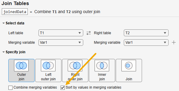
Join Tables Live Editor task, showing the check box for sorting output table rows by values in the merging variables

Create and work with datetime arrays in different time standards

You can now create and work with datetime arrays in International Atomic Time (TAI) and Terrestrial Time (TT), in addition to Coordinated Universal Time (UTC), by using the TimeStandard name-value argument and property. These time standards are useful in domains such as aerospace, astronomy, and telecommunications, where the simplified version of UTC representation, which does not account for leap seconds, is insufficient.

To specify a time standard, use the TimeStandard name-value argument with the datetime function.

t = datetime("now",TimeStandard="TT");

To convert the time standard of an existing datetime array, set the TimeStandard property to a new supported value.

t.TimeStandard = "TAI";

CLDR upgraded to version 46 with updated locale data for datetime arrays

The Common Locale Data Repository (CLDR) locale data is upgraded to version 46. The datetime data type uses CLDR locale data for localized names and locale-specific date and time formats. For more information, visit cldr.unicode.org.

Preserve end-of-month and end-of-quarter dates in arithmetic with calendarDuration values

In datetime arithmetic, calendarDuration values can now preserve end-of-month or end-of-quarter dates by using the ArithmeticMethod name-value argument. To create calendarDuration arrays that preserve month ends in arithmetic, use calendarDuration with ArithmeticMethod="endofmonth" or use calmonths. To create calendarDuration arrays that preserve quarter ends in arithmetic, use calendarDuration with ArithmeticMethod="endofquarter", or use calquarters.

If you load a calendarDuration array with the ArithmeticMethod property into an earlier MATLAB release (R2014b through R2026a), the earlier release ignores the ArithmeticMethod property, and the loaded calendarDuration array uses the default arithmetic method that preserves the day of the month when possible.

The caldiff and between functions now support datetime difference computations with respect to month ends and quarter ends. The isregular function now supports end-of-month and end-of-quarter regularity detection. Timetables with row times that occur at the end of each month or quarter can now be treated as regular, so you can create and manipulate timetable data more easily.

Specify naming rule for variables in grouped summary table

When using the groupsummary function with table or timetable input data, you can control how variables in the output table are named. Specify the VariableNamingRule name-value argument as "methodname" to use the names of the computation methods as prefixes (for example, mean_Var1 or myFun_Var1), or as "noprefix" to match the variable names in the input data (for example, Var1).

Also, in the Compute by Group task, when you specify a computation method as a function handle, the name of the corresponding output table variable now includes a prefix derived from the function name (for example, myFun_Var1). Previously, the prefix was a generic label with a number (for example, fun1_Var1).

Explicitly control whether to normalize polynomial query points

Specify the Normalize argument to explicitly control whether the polyfit function normalizes the query points before fitting a polynomial to the input data.

If you specify Normalize=true, polyfit centers the query points at 0 and scales them to a standard deviation of 1 before fitting. The returned polynomial coefficients and fit statistics are expressed in terms of the normalized query points x^=x−x¯σx .

Previously, normalization was controlled implicitly by the number of output arguments. For example, specifying a third output argument, as in [coeffs,~,centerScale] = polyfit(x,y,n), automatically normalized the query points. This syntax is still supported. However, using Normalize is recommended because it makes the normalization behavior explicit and independent of the number of output arguments.

Return cross-correlation or cross-covariance for nonnegative or nonpositive lags

You can return the cross-correlation or cross-covariance for only nonnegative or nonpositive lags by specifying the LagSelection argument with the xcorr or xcov function. Specify LagSelection as "nonnegative" to return values for lags from 0 to maxlag, or as "nonpositive" for lags from -maxlag to 0.

Compute cross-correlation or cross-covariance using sparse inputs

The xcorr and xcov functions now support sparse inputs. You can compute cross-correlation and cross-covariance using sparse inputs to significantly reduce memory usage and improve processing performance when the inputs contain many elements that are zero.

Return moving mean from moving standard deviation or variance computation

When using the movstd or movvar function, you can return the moving mean used to calculate the moving standard deviation or variance by specifying a second output argument.

Compute variance or standard deviation of integer input data

The var and std functions now accept input data of type int8, int16, int32, uint8, uint16, or uint32.

categorical Data Type: Find elements by pattern matching using matches, startsWith, endsWith, and contains functions

The matches, startsWith, endsWith, and contains functions now support categorical arrays as the input array. Use these functions to determine whether elements in a categorical array have category names that match, start with, end with, or contain a specified pattern.

Run Experiment Manager experiment and access result programmatically

You can now run an experiment and access a result from an experiment without opening the Experiment Manager app by using these functions:

  • runExperiment — Run an experiment and return an ExperimentResult object. If you have Parallel Computing Toolbox™, you can specify UseParallel="on" to run experiment trials simultaneously.

  • experimentResult — Retrieve an existing result of an experiment as an ExperimentResult object.

  • experimentTrial — Retrieve a trial from an existing result of an experiment as an ExperimentTrial object.

  • experimentNames — List the names of experiments in a MATLAB project.

  • experimentResultNames — List the names of existing results from an experiment.

You must create and configure your experiments using the Experiment Manager app.

Data Import and Export

 Read and write data using Google Sheets

You can read and write data directly from Google Sheets™ spreadsheets using existing functions, such as readtable, writetable, readmatrix, writematrix, readcell, writecell, readtimetable, writetimetable, and sheetnames. To access a Google Sheets spreadsheet, specify the spreadsheet URL or spreadsheet ID as the filename input.

For example, read a Google Sheets spreadsheet into a table.

url = "https://docs.google.com/spreadsheets/d/SPREADSHEET_ID";
T = readtable(url);

Write a MATLAB table to an existing Google Sheets spreadsheet.

T = table([1;2;3],["a";"b";"c"],VariableNames=["Row","Label"]);
writetable(T,url);

You can use the Sheet and Range name-value arguments to specify a particular sheet or cell range within the spreadsheet.

T = readtable(url,Sheet="Sheet2",Range="A1:D10");
writetable(T,url,Sheet="Results",Range="A1");

Before you can access Google Sheets from MATLAB, you must connect your Google® account to MATLAB using the Connections panel. For more information, see Read and Write Data from Your Google Account.

Create and manage Amazon S3 connections using Connections panel

You can now create, configure, and manage multiple Amazon S3 connections directly from the Connections panel in MATLAB. Previously, accessing remote data in Amazon S3 required configuring credentials programmatically. Using the Connections panel, you can interactively set up connections by specifying a bucket name, Amazon Web Services (AWS) access key ID, and secret access key. Optionally, you also can specify the session token (if you are using temporary security credentials), the endpoint, and the geographic region of your bucket.

To create an Amazon S3 connection, go to the Home tab, and in the Environment section, click the Connections button to open the Connections panel. Then, in the Available Connections section, click the Add button next to Amazon S3.

For more information, see Work with Remote Data.
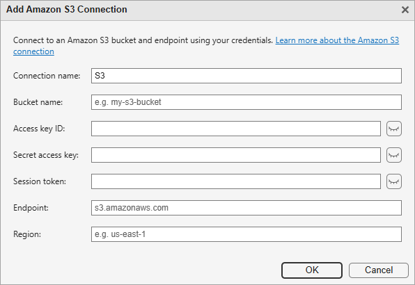
Add Amazon S3 Connection dialog box with text boxes for specifying a connection name, bucket name, access key ID, secret access key, session token, endpoint, and region

List file and folder names in natural order using dir

The dir function can now return folder contents in natural order using the SortOrder name-value argument. Natural order sorting treats numeric portions of filenames as numbers rather than characters. For example, listing = dir("ExampleFolder",SortOrder="natural") lists file2 before file10.

Specify S3 and Azure locations using https URLs

When you use MATLAB functions, such as readtable and writetable, to access remote data in Amazon S3™ and Azure® Blob Storage locations, you can now specify standard https:// URLs, in addition to existing support for the s3:// and wasbs:// schemes.

Resolve relative paths to absolute paths

The new resolveFilePath function returns the absolute paths of files and folders. Use this function to convert relative paths or partial paths to fully qualified absolute paths.

NetCDF functions support 64-bit data format

You can query, read, and write data from existing 64-bit data format (CDF-5) files using the netCDF functions. Create new 64-bit data format files using the netcdf.create function.

XSLT processor upgraded to Saxon 9b

The xslt function now uses the Saxon 9b XSLT processor.

Validate file information using new validation functions

Use these new validation functions to validate file information:

For more information about using validation functions for function argument and property checks, see Function Argument Validation and Property Validation Functions.

 Functionality being removed or changed

web function opens local files in HTML Viewer when MATLAB started with -nodesktop option

Behavior change

When you start MATLAB with the -nodesktop option and use the web function to open a local URL or file, the page now opens in the HTML Viewer. Previously, the page opened in a web browser.

xmlread function uses MAXP as the default XML processing engine

Behavior change

The xmlread function now uses the MATLAB API for XML Processing (MAXP) as the default XML processing engine. Previously, the xmlread function used the Java API for XML Processing (JAXP) by default. To specify JAXP, set the XMLEngine name-value argument to "jaxp".

serial function now errors

Errors

serial and its object properties now error and will be removed in a future release. Use serialport and its properties instead.

This example shows how to connect to a serial port device using the recommended functionality.

FunctionalityUse This Instead
s = serial("COM1");
s.BaudRate = 115200;
fopen(s)
s = serialport("COM1",115200);

For more information about updating your code to use the recommended functionality, see Transition Your Code to serialport Interface.

Mathematics

Generate random numbers using two new algorithms: "pcg" and "xoshiro"

You can use two new algorithms for random number generation.

NameAlgorithmMultiple Stream and Substream SupportDescriptionApproximate Period in Full Precision
"pcg"

"pcg64dxsm"

Yes64-bit permuted congruential generator with double xor-shift multiply2255 (263 streams of length 2192)
"xoshiro"

"xoshiro256pp"

YesXor-shift-rotate generator with 256-bit state and double addition2256 (264 streams of length 2192)

Both algorithms also provide the option to use full precision, and they use "Inversion" as the default normal transform.

To select these generator algorithms when controlling the MATLAB random number generator using the rng function, specify the generator name, such as rng("pcg") or rng("xoshiro"). You can also set either generator as the default by specifying it in the MATLAB Settings Window.

To select these generator algorithms when creating and controlling a random number stream using RandStream or RandStream.create, specify either the generator algorithm or its name, such as RandStream("pcg64dxsm") or RandStream("pcg").

 Additional support for RandStream object

The RandStream object has several improvements:

  • You can now create a copy of an existing random number stream with the same properties and state using the syntax s = RandStream(existingStream). When you generate random numbers using the newly copied stream and the existing stream, sampling from one stream does not affect the other.

  • When creating a RandStream object, you can choose whether to generate antithetic random numbers or whether to use full precision by specifying the Antithetic or FullPrecision name-value argument, respectively.

  • When using RandStream.list, you can now specify an output argument to return a table of all available generator algorithms. The table provides detailed information for each algorithm, including the generator name, multiple-stream support, and description.

 Compatibility Considerations

The RandStream object also has some changes in behavior:

  • For a random number stream that uses "Polar" as the normal transformation algorithm, saving and restoring the internal state of the stream now accurately reproduces the sequence of random numbers.

    For example, create a random number stream using the Mersenne Twister algorithm and the polar normal transformation. Generate a random number from this stream, and save the stream state before generating a second random number.

    s = RandStream("twister",NormalTransform="Polar");
    n1 = randn(s);
    savedState = s.State;
    n2 = randn(s)
    n2 =
       -0.7733
    Next, restore the stream state to the previously saved state. Generate a third random number. The second and third random numbers are the same.
    s.State = savedState;
    n3 = randn(s)
    n3 =
       -0.7733
    In previous releases, this code produced different values for the second and third random numbers.

  • Calling RandStream.list without an output argument now displays a table of all available generator algorithms with more detailed information about the generators, including their names and multi-stream support. In previous releases, RandStream.list displayed only the available generator algorithms and their descriptions.

Perform convolutions using sparse inputs

The conv, conv2, and convn functions now support sparse inputs. You can perform convolutions using sparse inputs to significantly reduce memory usage and improve processing performance when the inputs contain many elements that are zero.

Evaluate definite integral with variable upper limit

You can evaluate a definite integral with a variable upper limit using the new integralInterpolant object. You can also calculate the interpolated integral at values in the interval by querying the integralInterpolant object at a point or set of points.

Specify points of interest in integration region

You can specify points of interest, such as local extrema, in the integration region of a double or triple integral by specifying the Waypoints name-value argument of the integral2 and integral3 functions. The integrator uses the specified waypoints in the initial mesh.

Additional support for ordinary differential equations

The ode object and ODEResults object have new properties that you can use when solving ordinary differential equations:

  • You can specify the exact time values that you want the ODE solver to reach by setting the Waypoints property of the ode object. The solver reaches the specified time values by adjusting its step size.

  • You can calculate the Jacobian of a complex equation using automatic differentiation by setting the JacobianMethod property of the ode object to "autodiff".

  • You can identify why the integration of an ode object stopped by using the new StopReason property returned by the ODEResults object. The StopReason property indicates if the solver completed the integration, stopped the integration due to a specified function or event, or failed to meet specified tolerances during integration.

  • You can set a lower bound on the step size of any step taken by SUNDIALS ODE solvers by setting the MinStep property of matlab.ode.options.IDAS, matlab.ode.options.CVODESNonstiff, and matlab.ode.options.CVODESStiff objects, through the SolverOptions property of the ode object.

Graphics

Plot multiple data sets simultaneously with histogram, binscatter, geoplot, and other functions

Now you can use more plotting functions to visualize multiple data sets simultaneously:

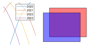
To accommodate multiple data sets, binscatter plots now support transparency. When you create multiple binned scatter plots, each distribution has a different overall hue by default, and transparency varies across the tiles according to the bin counts. If you plot one binned scatter plot, the plot is opaque and has the same appearance as in previous releases.

Histogram, binned scatter plot, and scatter plot in geographic coordinates, each displaying multiple data sets

Export figures as web canvases interactively

Create HTML files that contain interactive web canvases by selecting Save As > Export To in the figure toolstrip or by using the uiexportdlg function. In both approaches, select the HTML format option in the Export dialog box to export a figure as a web canvas.

Section of the Export dialog box with the updated list of format options, including HTML

For more information, see Print or Export Figure from Figure Toolstrip.

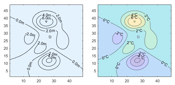
Configure semitransparent edges and meshes of function plots

Control the transparency level of the edges and meshes of function plots created with the fsurf, fmesh, and fimplicit3 functions by setting the EdgeAlpha property of the plot to a number between 0 and 1. A value of 0 makes the edges completely transparent and 1 makes the edges opaque.
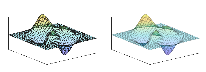
Two function surface plots with meshes that have different levels of transparency

Maximize geographic axes by filling available space

Maximize geographic axes by filling the available space within the parent container. To maximize the axes, set the MapLayout property of the GeographicAxes object to "maximized". Maximizing the axes hides the axis labels, ticks, tick labels, grid, and titles. The default for MapLayout is "normal", which displays the axes in a box that is inset from the edges of the parent container.

This image compares the normal map layout and the maximized map layout.

Comparison of normal and maximized map layouts

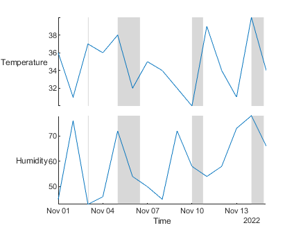
Display or hide axes toolbar in stacked plots and geographic bubble charts

Display or hide the axes toolbar in charts created with the stackedplot and geobubble functions by setting the ToolbarVisible property of the chart. The axes toolbar is visible by default, but you can hide it by setting the property to "off".

 Functionality being removed or changed

GraphicsSmoothing and FontSmoothing properties will be removed

Warns

MATLAB issues a warning if you set or get the value of the GraphicsSmoothing property of a figure or the FontSmoothing property of axes, rulers, and text objects. These properties will be removed in a future release. Since R2025a, all graphics and text are smooth regardless of the value of these properties.

MATLAB issues an error if you set or get the FontSmoothing property of a GeographicScalebar object.

plotyy will be removed

Still runs

The plotyy function will be removed in a future release. Use the yyaxis function instead.

The yyaxis function has several advantages over the plotyy function.

  • Unlike plotyy, the yyaxis function creates one Axes object with two y-axes. plotyy creates two overlaid Axes objects that can get out of sync.

  • You can use yyaxis with any 2-D plotting function, including functions with varied syntaxes, such as errorbar. By contrast, plotyy is limited to working with plotting functions of the form function(x,y).

This table shows some typical uses of plotyy and how to update your code.

Not RecommendedRecommended

plotyy(x1,y1,x2,y2)

yyaxis left 
plot(x1,y1) 
yyaxis right 
plot(x2,y2)

plotyy(x1,y1,x2,y2,'function1','function2')

yyaxis left 
function1(x1,y1) 
yyaxis right 
function2(x2,y2)

App Building

 Save App Designer apps in plain text file format to use with source control

You can save App Designer apps in a new plain text file format, which is useful for source control integration. The plain text app format consists of two files: an app code file (.m) and an app configuration file (.xml). Both files can be opened in App Designer and in other editors. For more information, see App Designer File Formats.

Add UI components to app canvas using quick insert menu

In App Designer Design View, you can add UI components to an app by double-clicking the app canvas and selecting a component from the quick insert menu. For more information, see Lay Out Apps in App Designer Design View.

Interactions with Code Browser and Property Inspector in App Designer have new keyboard shortcuts

In App Designer, you can now interact with the Code Browser and Property Inspector using new keyboard shortcuts. To move focus between tab headers, use the left and right arrow keys. When the intended tab is in focus, use the Tab key to navigate through the content.

In previous releases, there were no keyboard shortcuts to move focus between tab headers or navigate through content in the Code Browser or Property Inspector.

For more information, see App Designer Keyboard Shortcuts.

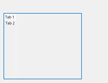
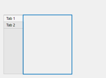
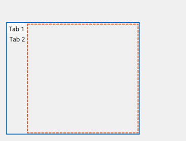
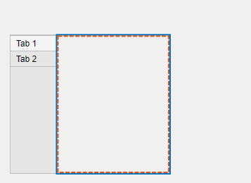
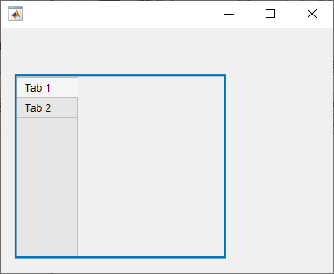
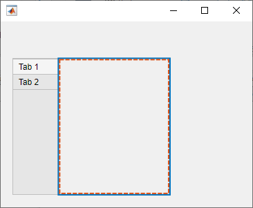
 Manage layout and exclusive selection of radio buttons or toggle buttons

For improved layout control, you can now parent radio buttons (created using uiradiobutton) and toggle buttons (created using uitogglebutton) directly to figures, tabs, panels, and grid layouts. Previously, radio buttons and toggle buttons had to be parented to button groups.

To manage the exclusive selection of a set of radio buttons or toggle buttons, create a selection group using the new uiselectiongroup function. For more information about selection groups, see SingleSelectionGroup.

 Compatibility Considerations

If you do not specify a parent container when creating a radio button or a toggle button, MATLAB now calls the uifigure function to create a new Figure object that serves as the parent container. Previously, uibuttongroup created the default parent container.

The default Position property value for radio buttons (created using uiradiobutton) is now [100 100 91 22]. Previously, the default value was [10 10 91 22].

The default Position property value for toggle buttons (created using uitogglebutton) is now [100 100 100 22]. Previously, the default value was [10 10 100 22].

Test apps using the new double-press gesture and updated existing gestures

The app testing framework introduces the double-press gesture and extends support for existing gestures:

 Functionality being removed or changed

Figures that have a menu bar or a toolbar no longer support desktop docking

Behavior change

Figures created using the figure function that have a menu bar or a toolbar no longer support docking into the MATLAB desktop. Figures created using the uifigure function that have a menu bar or toolbar still support docking into the desktop.

CurrentObject property of Figure updates on clicks and key presses

Behavior change

For a Figure object, MATLAB now sets the CurrentObject property to the last object selected in the figure, in response to both clicks and key presses. Previously, the CurrentObject property updated in response to clicks only.

Performance

 datetime Data Type: Improved performance with datetime arrays

Operations on datetime arrays show improved performance. These operations include but are not limited to:

  • Array creation

  • Array indexing

  • Reshaping

  • Converting different data types to datetime

For example, this code creates a datetime scalar. The code is about 11x faster than in the previous release.

function timingTest
for i = 1:1e5
    d = datetime(2026,1,1);
end
end

The approximate execution times are:

R2026a: 2.22 s

R2026b: 0.19 s

As another example, this code gets the size of a datetime vector. The code is about 43x faster than in the previous release.

function timingTest
d = [datetime("yesterday") datetime("today") datetime("tomorrow")];
for i = 1:1e5
    s = size(d);
end
end

The approximate execution times are:

R2026a: 0.32 s

R2026b: 0.0073 s

The code was timed on a Windows 11, AMD EPYC™ 74F3 24-Core Processor @ 3.19 GHz test system using the timeit function.

timeit(@timingTest)

 groupsummary Function: Improved performance with string grouping vector

The groupsummary function shows improved performance when the input data is a large, numeric variable or vector, the grouping variable or vector type is string, and you specify at least one of the "sum", "mean", "min", "max", "range", "nummissing", or "nnz" computation methods.

For example, this code computes the minimum, mean, and maximum for a 5,000,000-element numeric vector using a grouping vector of type string. The code is about 3.3x faster than in the previous release.

function t = timingTest
n = 5e6;
numGroups = 1e4;
A = rand(n,1);
groups = repmat(string(rand(numGroups,1)),n/numGroups,1);
G = @() groupsummary(A,groups,["min","mean","max"]);
t = timeit(G);
end

The approximate execution times are:

R2026a: 0.86 s

R2026b: 0.26 s

The code was timed on a Windows 11, AMD EPYC 74F3 24-Core Processor @ 3.19 GHz test system by calling the timingTest function.

innerjoin and outerjoin Functions: Improved performance for tall tables without sorting output rows

The innerjoin and outerjoin functions show improved performance when you join a tall table with an in-memory table without sorting the rows of the output table. For information on sorting, see the release note Specify row order of output table for inner and outer joins.

For example, these code blocks each perform an inner join of a tall table and an in-memory table and gather the joined table into memory. The R2026b code calls innerjoin with RowOrder="stable", which returns the output table without sorting the rows. For workflows that do not require sorted output, this approach is about 6.6x faster than the default sorted join behavior in R2026a.

R2026aR2026b
function t = timeInnerJoinWithTall
% Run tall code on the local MATLAB session
mapreducer(0);

% Create tall table
x = randi(1e3,1e4,1);
y = randi(1e3,1e4,1);
t = table((1:length(x))',x,y,VariableNames=["keys","Var1","Var2"]);
tallTable = tall(t);

% Create in-memory table
inMemoryTable = table(randperm(1e4,100)',x(1:100),y(1:100), ...
    VariableNames=["keys","Var3","Var4"]);

% Measure time for innerjoin
    function timeInnerJoin
        C = innerjoin(tallTable,inMemoryTable);
        gather(C);
    end
t = timeit(@timeInnerJoin);
end 
function t = timeStableInnerJoinWithTall
% Run tall code on the local MATLAB session
mapreducer(0);

% Create tall table
x = randi(1e3,1e4,1);
y = randi(1e3,1e4,1);
t = table((1:length(x))',x,y,VariableNames=["keys","Var1","Var2"]);
tallTable = tall(t);

% Create in-memory table
inMemoryTable = table(randperm(1e4,100)',x(1:100),y(1:100), ...
    VariableNames=["keys","Var3","Var4"]);

% Measure time for innerjoin
    function timeInnerJoin
        C = innerjoin(tallTable,inMemoryTable,RowOrder="stable");
        gather(C);
    end
t = timeit(@timeInnerJoin);
end 

The approximate execution times are:

R2026a: 0.53 s

R2026b: 0.08 s

The code was timed on a Windows 11, AMD® EPYC 9474F 24-Core Processor @ 3.6 GHz with 64 GB RAM test system by calling the timeInnerJoinWithTall and timeStableInnerJoinWithTall functions.

jsondecode Function: Improved performance when decoding JSON-formatted arrays

The jsondecode function shows improved performance when decoding JSON-formatted arrays containing mixed numeric and text data. For example, this code creates a JSON-encoded cell array where elements alternate between numeric and text data, and then decodes it. The call to jsondecode is about 1.2x faster than in the previous release.

function t = jsondecodePerformance
N = 1000*1000;
c = num2cell(randi([1 9],N,1));
c(2:2:end) = cellstr(string([c{2:2:end}]));
json = jsonencode(c);

f = @()jsondecode(json);
t = timeit(f);
end

The approximate execution times are:

R2026a: 0.36 s

R2026b: 0.30 s

The performance improvement is particularly noticeable for arrays of numeric data. For example, this code creates a JSON-encoded array of one million random integers and decodes it. The call to jsondecode is about 6x faster than in the previous release.

function t = jsondecodePerformanceIntegers
N = 1000*1000;
json = jsonencode(randi([1 9], N, 1));

f = @()jsondecode(json);
t = timeit(f);
end

The approximate execution times are:

R2026a: 0.54 s

R2026b: 0.09 s

The code was timed on a Windows 11, AMD EPYC 74F3 24-Core Processor @ 3.19 GHz test system by calling the jsondecodePerformance and jsondecodePerformanceIntegers functions.

dir Function: Improved performance when recursive listing of remote locations

The dir function shows improved performance when recursively listing the contents of remote storage locations, such as Amazon S3 buckets. For example, this code recursively lists all files in a remote Amazon S3 folder containing approximately 500 files and folders. The code is about 450x faster than in the previous release.

function t = timingTest
dir("s3://example_bucket/example_folder/**/*");
end

The approximate execution times are:

R2026a: 1045 s

R2026b: 2.3 s

The code was timed on a Windows 11, AMD EPYC 74F3 24-Core Processor @ 3.19 GHz test system using the timeit function. Execution times for remote operations also depend on network bandwidth, server load, and the number of files in the remote location.

timeit(@timingTest)

ismember Function: Improved performance with string query and set arrays

The ismember function shows improved performance when both the query and set arrays are of type string. The improvement is most noticeable when some elements of the query array are found in the set array.

For example, this code determines which strings in a 100-element string array are also in a 3,000,000-element string array. The code is about 3.9x faster than in the previous release.

function t = timingTest
A = string(rand(100,1));
B = repmat(string(rand(1e3,1)),3e3,1);
Lia = @() ismember(A,B);
t = timeit(Lia);
end

The approximate execution times are:

R2026a: 0.59 s

R2026b: 0.15 s

The code was timed on a Windows 11, AMD EPYC 74F3 24-Core Processor @ 3.19 GHz test system by calling the timingTest function.

islocalmin and islocalmax Functions: Improved performance

The islocalmin and islocalmax functions show improved performance. The improvement is most noticeable when you do not specify name-value arguments and you return only one output.

For example, this code finds the local maxima in a 50,000,000-element numeric vector. The code is about 3.4x faster than in the previous release.

function t = timingTest
A = rand(5e7,1);
f = @() islocalmax(A);
t = timeit(f);
end

The approximate execution times are:

R2026a: 1.00 s

R2026b: 0.29 s

The code was timed on a Windows 11, AMD EPYC 74F3 24-Core Processor @ 3.19 GHz test system by calling the timingTest function.

unique Function: Improved performance with string input data

The unique function shows improved performance when the input data type is string. For example, this code finds the unique values in a 2,000,000-element string array. The code is about 1.4x faster than in the previous release.

function t = timingTest
A = repmat(string(rand(1e3,1)),2e3,1);
C = @() unique(A);
t = timeit(C);
end

The approximate execution times are:

R2026a: 0.40 s

R2026b: 0.29 s

The code was timed on a Windows 11, AMD EPYC 74F3 24-Core Processor @ 3.19 GHz test system by calling the timingTest function.

polyshape Objects: Improved performance for Boolean operations with a single input

The union and intersect functions show improved performance when called with a single input, such as union(gv) and intersect(gv), where gv is a vector of polyshape objects.

For example, this code finds the union of 1000 polyshape objects. The call to union is about 94x faster than in R2025b.

function t = timingTest
basePoly = polyshape([0 1 0.5],[0 0 1]);
P = repmat(polyshape,1000,1);
rng(42);
for k = 1:1000
    P(k) = translate(basePoly,[50*rand,50*rand]);
end
Q = @() union(P);
t = timeit(Q);
end

The approximate execution times are:

R2025b: 1.316 s

R2026b: 0.014 s

The code was timed on a Windows 11, Intel Core® i9-14900K @ 3.20 GHz test system with 128 GB memory by calling the timingTest function.

nufftn Function: Improved performance for uniform-to-nonuniform transformations

The nufftn function shows improved performance when transforming data from uniformly spaced sample points to nonuniformly spaced query points.

For example, this code creates a 1,000,000-by-3 matrix of nonuniform query points F. The code then calculates the 3-D nonuniform discrete Fourier transform along each dimension of a 100-by-100-by-100 array X, transforming the data from the default uniform sample points to the nonuniform query points. The code is about 1.6x faster than in the previous release.

function t = timingQueryPoints
n = 100;
F = rand(n^3,3);
X = rand(n,n,n);

Y = @() nufftn(X,[],F);
t = timeit(Y);
end

The approximate execution times are:

R2026a: 1.00 s

R2026b: 0.64 s

The code was timed on a Windows 11, AMD EPYC 74F3 24-Core Processor @ 3.19 GHz test system by calling the timingQueryPoints function.

Create Plot Task: Improved performance when opening for the first time

The Create Plot task shows improved performance when opening for the first time in a MATLAB session. The delay between clicking Create Plot and the task being ready is reduced. Because the Create Plot task loads visualizations from your installed MathWorks® toolboxes and products, the improvement is most noticeable when many toolboxes and products are installed.

For example, for a set of installed toolboxes and products that loads 91 visualizations, you can use the task about 1.9x sooner than in the previous release.

The approximate rendering times are:

R2026a: 30 s

R2026b: 16 s

The action was timed on a Windows 11, AMD EPYC 74F3 24-Core Processor @ 3.19 GHz test system by inserting the Create Plot task into a live script.

uislider Function: Improved performance when resizing an app with multiple sliders in a grid

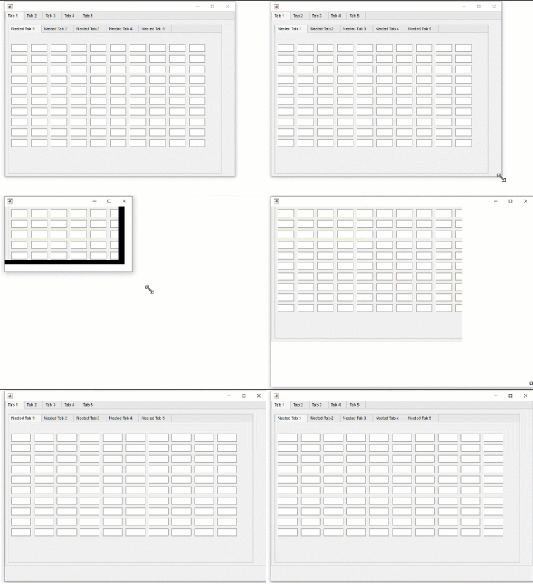
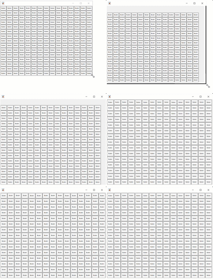
When you resize an app figure window that contains multiple sliders created using the uislider function and those sliders are in a grid layout manager, the app repositions its content faster in R2026b than R2026a.

For example, this code creates an app that contains 10 sliders in a grid layout manager and resizes the figure window. The code is about 1.5x faster than in the previous release.

function timingTest
f = uifigure;
g = uigridlayout(f,[5 2]);

for k = 1:10
    uislider(g);
end

widths = linspace(500,900,25);
heights = linspace(600,1000,25);
sizes = [widths(:),heights(:)];

for k = 1:size(sizes,1)
    f.Position(3:4) = sizes(k,:);
    drawnow;
end

close(f)
end

The approximate execution times are:

R2026a: 3 s

R2026b: 2 s

The code was timed on a Windows 11, AMD EPYC 74F3 24-Core Processor @ 3.19 GHz test system using the timeit function.

timeit(@timingTest)

plot and plot3 Functions: Improved responsiveness for large data visualizations

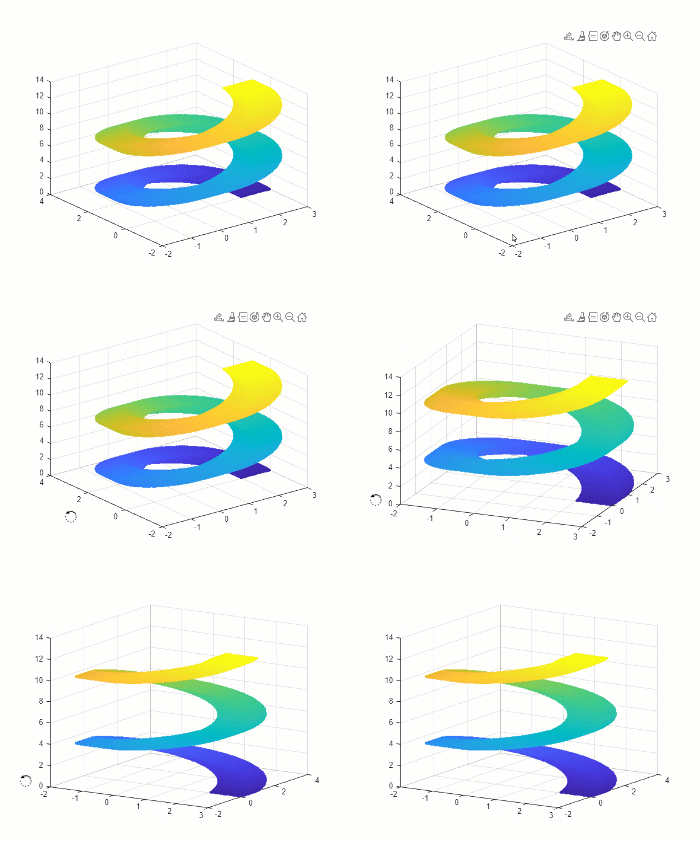
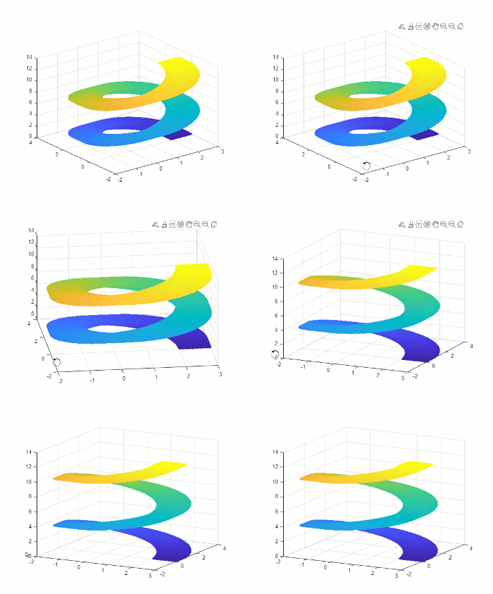
The plot and plot3 functions show improved responsiveness for large data sets by displaying lines and markers incrementally and showing a progress spinner in the figure tab until rendering is complete. This behavior provides a more responsive experience. Before R2026b, all the details display simultaneously after a longer period of time.

For example, on a Windows 11, AMD EPYC 74F3 24-Core Processor @ 3.19 GHz test system that has 65 GB of system memory and an NVIDIA A16-2B GPU with 2 GB RAM, this code begins drawing content in the figure approximately 1.4x faster than in the previous release.

rng(11);
numLines = 12;
dataSize = 5e7;
x = linspace(0,10,dataSize);
y = sin(x + linspace(0,pi,numLines)') ...
       +0.01*cumsum(randn(numLines,numel(x)),2);
figure
plot(x,y)

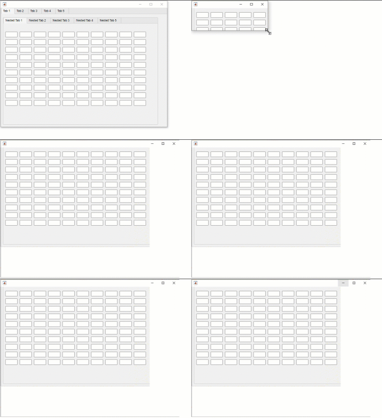
This video compares the delay between executing the plot command and the appearance of the plot in different releases. The left figure shows the R2026a behavior, and the right figure shows the R2026b behavior.

Improved stability and memory usage for batch processing figures

When you create multiple figure windows using batch mode, parallel workers (requires Parallel Computing Toolbox), or in a standalone executable, the figure windows now consume less memory than in previous releases. To further reduce memory usage, close any figures that you no longer need.

Continuous integration and continuous delivery (CI/CD) workflows that open and close large numbers of figures have improved stability and memory usage. As a result, you can run automated processes that involve opening and closing large numbers of figures for a much longer period of time.

Heterogeneous Class Hierarchies: Improved performance for method invocation

Invoking methods defined in heterogeneous class hierarchies shows improved performance. For example, the runMethodLoop function invokes the getValue method on hCircle and hSquare objects 1,000,000 times, and the loop is timed by the methodHeterogeneous function. The code is about 600x faster than in the previous release. (The full code for the heterogeneous hierarchy is listed at the end of this note.)

function runMethodLoop(obj)
    for j = 1:1e6
        out = obj.getValue();
    end
end
function methodHeterogeneous
    obj = [hCircle,hSquare];
    f = @() runMethodLoop(obj);
    t = timeit(f)
end

The approximate execution times are:

R2026a: 7.6 s

R2026b: 0.012 s

The code was timed on a Windows 11, Intel® Xeon® CPU W-2133 6-Core Processor @ 3.60 GHz test system.

The root class of the heterogeneous hierarchy is hShape, and hCircle and hSquare are subclasses. hCircle and hSquare both inherit the getValue method from hShape.

classdef hShape < matlab.mixin.Heterogeneous
    properties
        id = 1;
    end

    methods (Sealed)
        function out = getValue(obj)
            out = 3;
        end
    end
end
classdef hCircle < hShape
end
classdef hSquare < hShape
end

Heterogeneous Class Hierarchies: Improved performance for property access

Accessing properties defined in heterogeneous class hierarchies shows improved performance. For example, the runPropertyLoop function reads the value of property id in hCircle and hSquare objects 1,000,000 times, and the loop is timed by the propertyHeterogeneous function. To minimize overhead, runPropertyLoop accesses the properties by passing them as arguments to the function foo, which performs no operations on the values. The code is about 20x faster than in the previous release. (The full code for the heterogeneous hierarchy is listed at the end of this note.)

function runPropertyLoop(obj)
    for j = 1:1e6
        foo(obj.id)
    end
end
function propertyHeterogeneous
    obj = [hCircle,hSquare];
    f = @() runPropertyLoop(obj);
    t = timeit(f)
end

The approximate execution times are:

R2026a: 5.1 s

R2026b: 0.21 s

The code was timed on a Windows 11, Intel Xeon CPU W-2133 6-Core Processor @ 3.60 GHz test system.

The root class of the heterogeneous hierarchy is hShape, and hCircle and hSquare are subclasses. hCircle and hSquare both inherit the id property from hShape.

classdef hShape < matlab.mixin.Heterogeneous
    properties
        id = 1;
    end

    methods (Sealed)
        function out = getValue(obj)
            out = 3;
        end
    end
end
classdef hCircle < hShape
end
classdef hSquare < hShape
end
function foo(varargin)
end

validatestring Function: Improved performance

The validatestring function shows improved performance. For example, validating a partial string match against a list of options is about 5.8x faster than in the previous release.

function t = timingValidatestring
s = "omit";
opts = ["omitnan" "includenan"];

f = @() validatestring(s,opts);
t = timeit(f);
end

The approximate execution times are:

R2026a: 0.000150 s

R2026b: 0.000026 s

The code was timed on a Windows 11, AMD EPYC 74F3 24-Core Processor @ 3.19 GHz test system by calling the timingValidatestring function.

MATLAB Build Tool: Improved performance when plotting and running tasks

Plotting and running tasks in a build file show improved performance due to faster task dependency analysis by the build tool. In general, the improvements become more noticeable as the number of tasks and dependencies in the build file increases. The greatest improvements occur in build files with dependent task groups that contain a large number of tasks.

For example, suppose you have a build file with two task groups named "g1" and "g2", each containing 100 tasks, where the "g2" task group depends on the "g1" task group.

function plan = buildfile
import matlab.buildtool.Task

plan = buildplan;

plan("g1:t"+(1:100)) = Task;

plan("g2:t"+(1:100)) = Task;
plan("g2").Dependencies = "g1";
end

Plotting the tasks in the build file is about 4.8x faster than in the previous release. The approximate execution times are:

R2026a: 2.9 s

R2026b: 0.6 s

Running the tasks in the build file is about 1.5x faster than in the previous release. The approximate execution times are:

R2026a: 8.0 s

R2026b: 5.2 s

Plotting and running the tasks were timed on a Windows 11, Intel Xeon 6-Core Processor @ 3.60 GHz test system using the timeit function.

Plotting TasksRunning Tasks
timeit(@() plot(buildfile))
timeit(@() buildtool("g2","-verbosity",0))

MATLAB Editor: Improved scrolling on high-DPI displays

Scrolling in the MATLAB Editor is smoother on high-DPI displays. When you scroll using the scrollbar on Windows systems with display scaling above 100% or on macOS systems, line numbers and code content move together. In previous releases, line numbers might visibly lag behind the code while scrolling.

For example, on a Windows 11, Intel Xeon W-2133 6-Core Processor @ 3.60 GHz test system with 64 GB RAM, if you set display scaling to 150%, open any file in the Editor, and scroll using the scrollbar, the line numbers and code update together.

This video compares the lag between the line numbers and code content while scrolling in different releases. The left side shows the R2026a behavior, and the right side shows the R2026b behavior.

Software Development

 Save projects in TOML format for easier review and editing

The new matlab.toml definition file type allows you to define and manage your entire project configuration in a single TOML file. This format is easier to review and merge under source control, and you can edit it directly in the MATLAB Editor.

With a TOML-based project, you can:

  • Manage project configuration, package dependencies, and file labels in one place.

  • Declare dependencies on MATLAB packages with version constraints, and automatically install them from configured repositories when the project opens.

  • Associate labels with file patterns so that matching files are labeled automatically.

  • Validate the TOML file to identify issues such as invalid syntax, invalid data, or missing files.

  • Detect missing package dependencies when running project checks.

To set the TOML format as the definition file type when you create a project, on the Home tab, in the Environment section, click Settings. Select MATLAB > Project and, in the New Projects section, set Project definition files to matlab.toml.

To convert an existing project to TOML format, use one of these methods:

  • On the Project tab, in the Environment section, click Settings. Then, in the Advanced section, edit Definition file type by clicking Change and selecting matlab.toml.

  • Use the matlab.project.convertDefinitionFiles function.

You can add package dependencies from the project settings, from the Dependencies tab, or by editing the matlab.toml file directly.

For more information, see:

 Share and install packages through File Exchange

MathWorks File Exchange is now a package repository, and add-ons installed from File Exchange are installed as packages. File Exchange is on the list of known repositories by default. You can remove File Exchange from the known repository list using mpmRemoveRepository and add it again using mpmAddRepository. To get the File Exchange URL known to MATLAB, use the matlab.mpm.FileExchange function.

Share and install packages with custom repositories using MATLAB package repository service

A MATLAB package repository service acts as an intermediary between the MATLAB Package Manager and your organization's artifact management system (such as JFrog Artifactory). Set up a custom repository by following the steps outlined here, Distribute Packages Using MATLAB Package Repository Service.

Check projects with greater scope and in the background

When you run project checks, you now have the option to run the checks for the top-level project as well as all its referenced projects. For more information, see Run Project Checks.

You can also run project checks in the background. If you enable this option, when an event that triggers a background check occurs, MATLAB queues this check and runs all queued checks after a specified delay. For more information, see Configure Global MATLAB Projects Settings.

Identify project tests at the folder level

You can now mark folders in your project as test folders. The MATLAB unit testing framework uses these test folders to quickly identify and run tests in the project. For more information, see Add Test Folders.

Move project files and match names with functions more easily

You can move files and folders within a project, into a project, or out of a project by using the moveFile function. The function also allows you to rename files and folders.

To match files and folders more efficiently, the findFiles, listRequiredFiles, and listImpactedFiles functions now support glob patterns for specifying files. You can use these glob patterns:

  • * — Match any characters within a single folder (nonrecursive wildcard).

  • ** — Match files and folders recursively.

  • ! — Exclude matches when used as a negation prefix.

  • / — Match directories only when used as a trailing slash.

Specify project shortcut names and groups programmatically

You can programmatically define the names and groups of your project shortcuts by specifying the Name and Group name-value arguments of the addShortcut function.

Filter project list to see files under source control

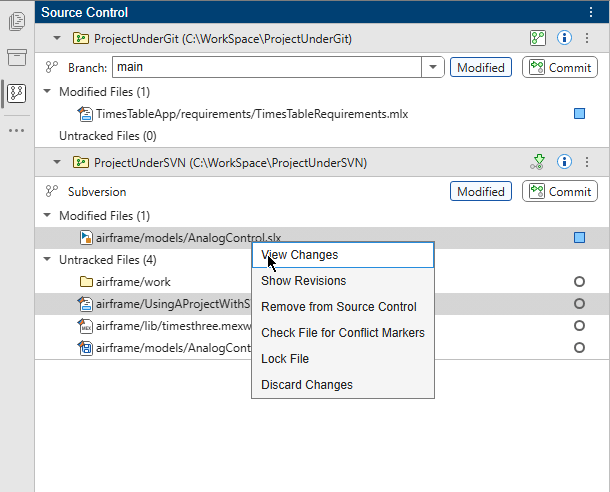
In the Project panel, you can filter files under the project root folder to view only the files that are tracked by source control. For more information, see Manage Project Files.

Projects created in empty folders have src and tests folders

When you create a new project in an empty folder, MATLAB now automatically adds the src and tests folders to the project. MATLAB does not add these folders if you create a project using the matlab.project.createProject function.

When you create a new project in any folder, you can also choose to initialize a Git™ repository.

Manage GitHub and GitLab connections from MATLAB

You can manage GitHub® and GitLab® connections directly from the MATLAB Connections panel. From the Connections panel, you can:

  • Manage GitHub or GitLab authentication.

  • Use one authentication workflow for GitHub or GitLab operations, including clone, fetch, push, and share.

  • Use multiple GitHub or GitLab accounts and link them to specific repositories.

  • Store authentication tokens securely in the MATLAB vault.

For more information, see Connect to GitHub or GitLab from MATLAB.

View pull requests and merge requests in MATLAB and share links to them

Use the Pull Requests panel to view and work with GitHub pull requests and GitLab merge requests directly within MATLAB.

  • View GitHub pull requests and GitLab merge requests without leaving MATLAB.

  • Compare files that changed in a pull or merge request, including Simulink® models.

  • Check out pull or merge requests locally to review and test changes.

  • Generate a shareable link to open GitHub pull requests or GitLab merge requests directly in a locally installed version of MATLAB.

For more information, see View and Share Pull Requests in MATLAB.

You can also generate links to view individual files on GitHub or open them in MATLAB Online™. In the Files panel, right-click the file you want to share and select Share > GitHub link or Share > Open GitHub file in MATLAB Online.

Custom MATLAB toolboxes are now called packages

The MATLAB language feature known as a toolbox is now a package, and the associated installation file (.mltbx) is now a package file. Packages are collections of code bundled for distribution. As of R2026b, the terminology is updated in both the documentation and software.

Package installation is handled by MATLAB Package Manager, which provides robust dependency management. MATLAB Package Manager is backward compatible with toolboxes created before R2026b. These toolboxes are supported and installed as packages.

You can interactively build a package in two ways:

  • If your code is in a MATLAB project, convert the project to the new TOML format, which enables the project to depend on packages. Open the project, go to the Project tab, and in the Tools section, click Build Package. MATLAB creates a package task with the same name as your project and opens it in the document area of the desktop.

  • If your files are not already included in a project, go to the Home tab, and in the Environment section, select Add-Ons > Build Package. Click Browse to select the folder containing your package files and then click OK. MATLAB creates a new project containing your files and a package task for configuring your package. If the folder you select already contains a project, the existing project is used instead. Configure the project to use the recommended TOML format.

To support MATLAB Package Manager functionality, the matlab.addons.toolbox.ToolboxOptions object includes three new properties: PackageName, PackageDependencies, and Readme.

For more information, see Share and Distribute Software.

Updates to support for packages

Packages have several improvements. You can:

  • Add custom labels — To make your package more easily searchable in repositories, including File Exchange, you can add custom package labels by using the Tags properties of the matlab.mpm.Package and matlab.addons.toolbox.ToolboxOptions objects.

  • Update installed packages — To update one or more installed packages to the latest available version or to a specific version, use the new mpmupdate function.

  • View changes before installation — To verify changes before you install a package, you can call mpminstall with the new DryRun name-value argument to see a list of all packages and dependencies to be installed, without installing them. If you also specify AllowVersionReplacement=true, then packages to be removed are displayed as well.

  • Add BSD license — To generate a BSD (Berkeley Software Distribution) license when building a package file (.mltbx), set the UseLicenseBSD property of the matlab.addons.toolbox.ToolboxOptions object. The UseLicenseBSD property must be true for package files uploaded to File Exchange.

Packages include extensions.json file

Packages built interactively or using matlab.addons.toolbox.packageToolbox now include an extensions.json file. This file is created during the build process if one does not exist.

MATLAB populates the extensions.json file using matlab.addons.toolbox.ToolboxOptions properties. The ToolboxImageFile property registers the package image. The AppGalleryFiles property determines app files registered with the apps gallery. The ToolboxGettingStartedGuide property registers the Getting Started guide.

Package installation logged by system audit logger

Package installation events are now logged by the system audit logger. MATLAB records the following information for each installed package and dependency:

  • Package ID

  • Originating repository

  • Download URL

  • Download destination

  • Package digest, as returned by digest

Audit logger behavior varies by operating system. On Windows, system audit logging must be enabled. Open a Windows PowerShell command prompt as an administrator and run these commands:

$source = "MathWorks"
$logName = "Application"
$eventSourceExists = [System.Diagnostics.EventLog]::SourceExists($source)

if (-not $eventSourceExists) {
    [System.Diagnostics.EventLog]::CreateEventSource($source, $logName)
    Write-Host "Event source $source created successfully."
} else {
    Write-Host "Event source $source already exists."
}

You can then specify the severity level to log by creating a new REG_DWORD value in the event source HKEY_LOCAL_MACHINE\SYSTEM\CurrentControlSet\Services\EventLog\Application\MathWorks. Set the REG_DWORD value to 0 to disable logging, 1 to log only critical events, 4 to log notice-level events, or 7 to log events at all severity levels.

On Linux and macOS systems, audit logging is on by default. You can disable audit logging or set the logging level by creating a file named /etc/mathworks/settings.json on Linux and /Library/Preferences/SystemConfiguration/MathWorks/settings.json on macOS with this code:

{
  "auditlogging": {
    "level": "all"
  }
}

Set the level property to "none" to disable logging, "critical" to log only critical events, and "all" to log all events.

Specify files and folders for Code Analyzer to ignore during analysis

Configure the Code Analyzer to ignore specific files and folders during analysis by using the "ignoredFiles" property in a Code Analyzer configuration file. For more information, see Customize Code Analyzer Checks Using Configuration File.

 Improved data model for build plan elements

The new matlab.buildtool.PlanElement class defines the minimal shared identity for all elements that you can add to a build plan, such as tasks and task groups. The matlab.buildtool.Task and matlab.buildtool.TaskGroup classes now derive from the PlanElement class and inherit its Name and Description properties.

 Compatibility Considerations

The new data model results in these changes:

  • The Tasks property of the matlab.buildtool.Plan class represents plan elements as a PlanElement vector. In previous releases, the property contains a Task vector instead.

  • The TaskGroup class is no longer a subclass of the Task class. Therefore, TaskGroup no longer includes the properties that are unique to the Task class, such as Actions, Inputs, and Outputs.

Speed up builds with task output caching

You can use task output caching in your builds by specifying the new -outputCache option with the buildtool command. When an output cache is available, the build tool skips tasks that can reuse outputs from earlier builds, improving build performance. For more information, see Cache Task Outputs.

Build package from TOML project by using built-in task class

You can build a package from a TOML project by using the matlab.buildtool.tasks.PackageTask class. A task created from the PackageTask class automatically uses the configuration in the matlab.toml project definition file. For an example, see Build Package from TOML Project.

Generate build reports in HTML format

You can generate an HTML build report by using the generateHTMLReport method of the matlab.buildtool.BuildResult class or the -report option of the buildtool command. The build report provides detailed information about the build, including the build environment, build summary, and individual task results.

Run tests using external parameters in MATLAB builds

You can inject new data into parameterized tests by using the ExternalParameters property or task argument of the matlab.buildtool.tasks.TestTask class. For an example, see Run Tests Using External Parameters.

Visually identify cyclic task dependencies in build task plots

You can visually identify cyclic task dependencies by using the plot method of the matlab.buildtool.Plan class. After plotting your tasks as a dependency graph, verify that the graph is acyclic. If the graph contains cycles, update your build plan to remove the cyclic dependencies.

In previous releases, the method throws an error and does not create a task graph if the build plan contains cyclic dependencies.

Emit MATLAB build telemetry data

You can instrument your MATLAB builds with OpenTelemetry™ to emit traces and metrics to observability backends. For more information, see Emit MATLAB Build Telemetry Data with OpenTelemetry Integration.

Test code insertion options in the Editor are goal oriented

The code insertion options in the Test section on the Editor tab now align with test authoring goals rather than programming concepts such as methods and properties. You can use these improved options to add tests to your test class and to specify setup code for individual tests or for the entire test class. For more information, see Insert Test Code Using Editor.

Use Test Browser when running tests with runtests function

You can now use the Test Browser app when running tests with the runtests function. To run tests and display results using the test browser, specify the UseTestBrowser name-value argument of the function as true.

If you run tests interactively from the Run Tests section on the MATLAB Toolstrip with the Use Test Browser option selected, the testing framework displays the command it uses to run the tests, including the UseTestBrowser name-value argument. For more information, see Run Tests in Editor.

Add source code to Test Browser for coverage reporting by dragging files and folders

You can add source code to the Test Browser app for coverage reporting by dragging source files and folders from the Files or Project panel into the Source pane. To access the Source pane, click the Open coverage settings button on the Test Browser toolbar, and then select Enable coverage reporting.

 Run tests in parallel with additional control

You now have more control over when to use a parallel pool to run tests using the runtests function. The UseParallel name-value argument of the function now accepts new "off", "auto", and "on" values. Specify UseParallel as "auto" to automatically use a parallel pool if one is available or as "on" to always use a parallel pool.

 Compatibility Considerations

Starting in R2026b, specifying the UseParallel name-value argument as true or false is not recommended. For more information, see Logical values for UseParallel argument of runtests function are not recommended.

Unit testing framework discovers tests in project test folders

The unit testing framework now discovers and runs tests in project test folders. In XML projects that define tests using both test folders and the Test classification label on files, the framework includes tests from both sources in the test suite. In TOML projects, test folders are the only way to define tests. For more information, see Identify and Run Tests in MATLAB Projects.

Create preformatted diagnostics for constraints in unit tests

You can create preformatted constraint diagnostics using the convenience methods of the matlab.unittest.constraints.Constraint and matlab.unittest.constraints.BooleanConstraint classes:

  • To create preformatted diagnostics inside the getDiagnosticFor method, use the createPassingDiagnostic and createFailingDiagnostic convenience methods of the Constraint class.

  • To create preformatted diagnostics inside the getNegativeDiagnosticFor method, use the createNegativePassingDiagnostic and createNegativeFailingDiagnostic convenience methods of the BooleanConstraint class.

The convenience methods automatically set the matlab.unittest.diagnostics.ConstraintDiagnostic object properties required to display the diagnostic information. For an example, see Create Custom Boolean Constraint.

Create UI figure using built-in test fixture

You can use the new matlab.unittest.fixtures.UIFigureFixture class to construct fixtures for creating a UI figure. For an example, see Create UI Figures for Testing.

Test apps using the new double-press gesture and updated existing gestures

The app testing framework now includes the double-press gesture and extends support for existing gestures:

 Functionality being removed or changed

Calling mpminstall with Force=true installs specified packages and dependencies even if it breaks existing dependencies

Behavior change

If you call mpminstall with Force=true, and if a dependency of the installed package conflicts with an already installed package or dependency, then the newly installed dependency overwrites the installed package or dependency even if it breaks an installed package.

For example, if installed packageA depends on version 1.0.0 of packageB and you call mpminstall with Force as true on packageC, which depends on version 2.0.0 of packageB, then mpminstall overwrites version 1.0.0 of packageB with version 2.0.0 and breaks the dependency of packageA.

In previous releases, mpminstall does not overwrite installed packages or dependencies if it would break the dependency of another installed package.

Package installation folder name is derived from PackageName property

Behavior change

When you install a package file (.mltbx), MATLAB creates a new folder in the designated installation area for the contents of the package. Starting in R2026b, MATLAB derives the name of this folder from the PackageName property of the corresponding matlab.addons.toolbox.ToolboxOptions object.

In previous releases, MATLAB derived the name of this folder from the ToolboxName property.

ToolboxVersion property of ToolboxOptions object must adhere to semantic version syntax

Behavior change

The ToolboxVersion property of the matlab.addons.toolbox.ToolboxOptions object must adhere to semantic version syntax. ToolboxVersion syntax follows the Semantic Versioning 2.0.0 format: <major>.<minor>.<patch>, where each version number must be a nonnegative integer, for example, 1.2.3. You can optionally specify a pre-release version by adding -<pre-release version> to the end of the version, for example, 1.2.3-alpha. Optionally specify a build version by adding +<build version>. Previously, the ToolboxVersion property accepted any text value without checking its format.

Description and RequiredAddons properties of ToolboxOptions object are no longer supported

Still runs

The Description and RequiredAddons properties of the matlab.addons.toolbox.ToolboxOptions object are no longer supported. Instead, use the Readme property to direct your package users to a file containing information about your package. Use the PackageDependencies property to define packages that your package depends on.

Logical values for UseParallel argument of runtests function are not recommended

Still runs

Starting in R2026b, for the runtests function, specifying the UseParallel name-value argument as true or false is not recommended. Use the "off", "auto", and "on" values instead.

This table shows how to update your code depending on your goal.

GoalNot RecommendedRecommended
Run tests in serial.runtests(UseParallel=false)runtests(UseParallel="off") (default)
Run tests in parallel, or if a parallel pool is not available, run them in serial.runtests(UseParallel=true)runtests(UseParallel="auto")
Run tests in parallel and error if a parallel pool is not available.N/Aruntests(UseParallel="on")

There are no plans to remove support for the true and false values.

Rerunning failed tests uses a default test runner if the original runner no longer exists

Still runs

When you rerun failed tests using the rerun link in the test summary, the testing framework uses a default test runner instead of the original runner if you ran tests using one of these options:

  • A nondefault test runner created with the testrunner function or one of the static methods of the matlab.unittest.TestRunner class and that test runner no longer exists

  • The run method of the matlab.unittest.TestCase class

In previous releases, the framework reruns failed tests using the original test runner.

External Language Interfaces

  Call Java from MATLAB: Install OpenJDK JRE Runtime

MATLAB no longer includes Java Runtime as part of its installation. For information about installing OpenJDK, see Configure Your System to Use Java.

MATLAB now supports OpenJDK 25 Java from https://adoptium.net/. For supported version information, see MATLAB Interfaces to Other Languages.

 Compatibility Considerations

Before R2026b, if you call jenv or matlab_jenv with the Java version argument set to "factory", MATLAB set the Java path to the version included with MATLAB. Starting in R2026b, MATLAB no longer includes Java as part of its installation, and the argument value "factory" is the same as "system", which represents the default Java version on your system. Likewise, the JavaEnvironment Configuration property value "factory" is the same as "system", which represents the default Java version on your system.

Call C++ from MATLAB: Programmatically publish MATLAB interface to C/C++ libraries

You can programmatically configure and publish MATLAB interfaces to C/C++ libraries by using objects in the clibgen.api namespace. Use this approach instead of editing library definition files when you want to modify a library interface. By defining the interface in MATLAB code, you can reuse the same definition across platforms and build environments, resulting in a more maintainable and repeatable published interface.

Call MATLAB from C++: Pass custom C++ structures to MATLAB functions

You can pass custom C++ structures directly to MATLAB functions from a C++ engine application. Previously, you had to manually convert structure fields to matlab::data::StructArray objects. Instead, pass pointers to your native C++ structures as arguments to matlab::engine::MATLABEngine::feval and receive structure pointers as outputs.

To pass custom C++ structures directly to MATLAB, you must start MATLAB using IN_PROCESS mode. For more information, see Pass C++ Structures to MATLAB Functions.

REST Function Service: Call MATLAB functions remotely from Python using REST services and native Python data types

The Python® class matlab.rest_function_service.client.MWHttpClient creates an object for calling MATLAB functions in a REST function service. Use this object in your Python client applications to pass inputs to MATLAB functions and receive outputs using native Python data types. For more information, see Call MATLAB Functions from Python Using REST.

Call Python from MATLAB: Install Python version 3.13 from Add-Ons panel

Use the MATLAB Support for Python 3.13 add-on to install a version of Python that is compatible with MATLAB R2026b. For details on installing this add-on, see Install and Configure Python for Use in MATLAB.

For a list of additional MATLAB releases that support Python 3.13, see Versions of Python Compatible with MATLAB Products by Release.

Call Python from MATLAB: Interrupt out-of-process execution using Ctrl+C

When calling Python from MATLAB in out-of-process execution mode, you can now press Ctrl+C to interrupt long-running or unresponsive Python code and terminate the process. For more details about out-of-process execution mode, see Out-of-Process Execution of Python Functionality.

 Support for Python version 3.14

MATLAB now supports Python version 3.14, in addition to versions 3.10, 3.11, 3.12, and 3.13. For supported version information, see Versions of Python Compatible with MATLAB Products by Release.

 Compatibility Considerations

For more information about changes to Python support, see Python version 3.9 is no longer supported.

Support for .NET 8 or higher

MATLAB supports .NET 8 or higher, in addition to existing support for the Microsoft® .NET Framework. For more information about changes to .NET support, see MATLAB Interfaces to Other Languages.

Support for Perl 5.42.2 and Perl 5.44.0 on Windows

As of R2026a (May 2026), the version of Perl included with MATLAB for Windows is updated to Perl 5.42.2. In addition, as of R2026b, the version of Perl included with MATLAB for Windows is updated to Perl 5.44.0.

If you use the perl command on Windows, see https://www.perl.org/ for information about using this version of Perl.

Compiler support for Intel oneAPI 2026

MATLAB supports Intel oneAPI 2026 with Microsoft Visual Studio® 2026 for C and C++ compilers for building C and C++ interfaces, MEX files, and standalone MATLAB engine and MAT-file applications on Windows.

 Functionality being removed or changed

Python version 3.9 is no longer supported

Errors

Support for Python version 3.9 is discontinued. For continued support for your applications, upgrade to a supported version of Python. For supported version information, see Versions of Python Compatible with MATLAB Products by Release.

usejava and javachk functions will no longer support "awt" and "swing" options

Still runs

The "awt" and "swing" options for the feature argument of the usejava and javachk functions will be removed in a future release. To detect Java, call usejava("jvm"). To detect the desktop, call desktop("inuse").

matlab.wsdl.createWSDLClient and matlab.wsdl.setWSDLToolPath have been removed

Errors

The matlab.wsdl.createWSDLClient and matlab.wsdl.setWSDLToolPath functions have been removed.

Use the MATLAB RESTful functions (webread and webwrite) or the MATLAB HTTP interface instead. For more information, see Call Web Services from MATLAB Using HTTP.

Hardware Support

Arduino Hardware: Support for Raspberry Pi Pico 2 and Pico 2 W boards

You can now use MATLAB Support Package for Arduino® Hardware in the installed version of MATLAB to communicate with the Raspberry Pi® Pico 2 boards over USB and the Pico 2 W boards over USB and Wi-Fi®. For more information, see Supported Boards.

Arduino Hardware: Support for ESP32-S3-DevKitC boards

You can now use MATLAB Support Package for Arduino Hardware in the installed version of MATLAB to communicate with ESP32-S3-DevKitC boards over USB, Bluetooth®, and Wi-Fi. For more information on how to configure ESP32 boards, see Set Up and Configure ESP32 Hardware.

You cannot use the support package to connect these boards with an Adafruit® Motor Shield V2, motor carrier, CAN interface, or serial devices. The function playTone and the name-value argument AnalogReferenceMode of the arduino object in external mode do not support these boards. For more information, see Supported Boards.

Arduino Hardware: Install Arduino-compatible libraries more easily

You can now use the arduinoio.customLibrary.downloadLibrary function to install Arduino-compatible libraries by specifying the library name, a GitHub® repository URL, or a local ZIP file. In each case, the function installs the library and returns the full path to the installed library folder.

Arduino Hardware: Create custom library template using arduinoio.customLibrary.createLibraryTemplate function

You can now use the arduinoio.customLibrary.createLibraryTemplate function to get started with creating a custom library.

The function generates a folder containing MATLAB and C++ templates for defining a custom library and establishing communication with Arduino hardware. You can then modify the templates to implement your own custom functionalities.

R2026a

New Features, Bug Fixes, Compatibility Considerations

Environment

 MATLAB Desktop: Share files in MATLAB Drive from MATLAB

You can now share a file stored in MATLAB Drive™ directly from MATLAB. When you share the file, MATLAB shares the folder that contains the file as well. Sharing files that are in the root MATLAB Drive folder is not supported.

To share a file, right-click the file in the Files panel, select Share, and then select from the available options. To manage permissions, select Invite Members and then add members with read or edit permissions to your file. To share your file with others through a link, select Create Link.

You also can now manage an already shared folder from inside that shared folder. To manage an existing shared folder, right-click any subfolder or white space inside the shared folder, select Share, and then select from the available options.

For more information, see Share Files Using MATLAB Drive.

 Java Runtime: Install your own version of Java

MATLAB provides two-way integration with the Java programming language and supports specific OpenJDK long-term support (LTS) releases across all platforms. After installing MATLAB, you can install OpenJDK using the Add-On Explorer:

  1. On the MATLAB Home tab, in the Environment section, click Add-Ons.

  2. In the Add-On Explorer, search for OpenJDK.

  3. Install the MATLAB Support for OpenJDK add-on.

  4. In the MATLAB Command Window, clear the current JRE™ so that MATLAB uses the installed OpenJDK add-on.

    jenv -clear

Alternatively, you can download and install any compatible OpenJDK distribution from https://adoptium.net/. For information about supported versions, see Versions of OpenJDK Compatible with MATLAB by Release.

In a future release, MATLAB will no longer include Oracle® Java as part of its installation. For additional details, see Java Runtime will no longer be installed by default in a future release.

 Live Editor Text: Create multilevel lists

You can create multilevel bulleted or numbered lists in live scripts or functions. To create a multilevel list, with your cursor in a text line, go to the Live Editor tab and in the Text section, click the Bulleted list or Numbered list button. Then, press the Tab key to indent a numbered or bulleted item.

To decrease the indentation, press Shift+Tab. To change a sublist to a different list type, use the Bulleted list and Numbered list buttons.

For more information, see Format Text in the Live Editor.
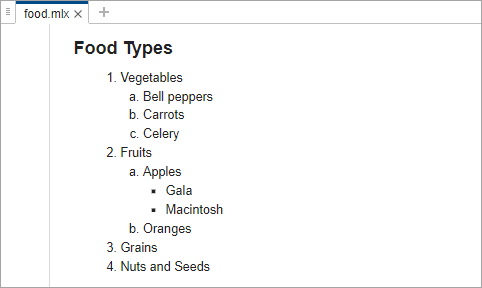
Live script showing a multilevel list of food types, including vegetables, fruits, grains, and nuts and seeds

MATLAB Desktop: Access recent files and online training using MATLAB Home page

The new MATLAB Home page gives you quick access to your recent files, online training, and other resources. To open the MATLAB Home page, in MATLAB, click the MATLAB Home button to the left of the Home tab.

MATLAB Home page with a Recent section containing a search box for searching recent files and folders and a list of five recent files, as well as an Online Training section containing two online training courses. The left pane contains links to additional resources, such as documentation, MATLAB Answers, and blogs.

Live Editor Controls: Run custom code on button click

You can specify code to run when a button control is clicked in a live script. To specify the code to run, right-click the button control in the live script and select Configure Control. Then, in the Execution section, set the Run option to User-defined code and enter the code to run. When the button is clicked, the specified code runs in the Command Window.

For more information, see Add Interactive Controls to a Live Script.

Live Editor Controls: Populate slider and spinner values using additional variable types

You can now populate the minimum, maximum, step, and default values for a slider or spinner using values stored in a variable of any numeric type. Previously, only variables of type double were supported.

For more information, see Link Variables to Controls.

Live Editor Tasks: Manage custom Live Editor tasks from the task gallery

Manage a custom Live Editor task from the task gallery, including configuring task metadata, opening the task class definition file, and removing the task from the task gallery and from code suggestions. To view these options, hover over the Live Editor task icon in the task gallery.
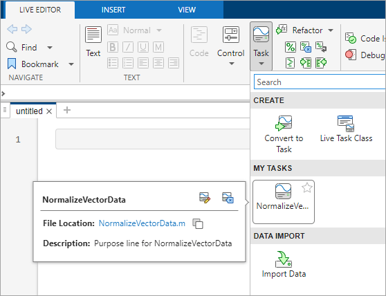
Live Editor task gallery showing the NormalizeVectorData custom task and options to configure the task metadata, remove the task, and open the class definition file

Editor Spell Checker: Check spelling in MATLAB code and Markdown files by default

Spell checking is now on by default in the Editor and Live Editor. If a file contains many unrecognized words, such as when not written in US English, MATLAB automatically turns spell checking off for that file. In addition, spell checking is now supported in Markdown files.

To turn spell checking off by default, on the Home tab, in the Environment section, click Settings. Select MATLAB > Editor/Debugger > Spelling and set Check spelling to Off. To change what text to spell check, in the Where to check spelling section, select or clear the available options.

For more information, see Editor/Debugger Spelling Settings.

Editor Files: Change the default end-of-line sequence for new files

By default, the end-of-line sequence for new files on Windows is the carriage return and line feed characters (\r\n). On Linux and macOS, the default end-of-line sequence for new files is the line feed character (\n).

To change the default end-of-line sequence, go to the Home tab, and in the Environment section, click Settings. Select MATLAB > Editor/Debugger, and then select an option for Default end of line sequence.

For more information, see General Settings for the Editor/Debugger.

Editor Comments: Enhanced support for wrapping comments containing non-ASCII characters

The Editor and Live Editor now wrap comments containing non-ASCII characters, including emojis and CJK (Chinese, Japanese, and Korean) characters, more accurately and intuitively. Wrapped comments maintain proper alignment and readability, regardless of character width or encoding.

Comparison Tool: Compare folders and ZIP files using improved interface

Compare folders and ZIP files using an improved interface. Improvements include quick filters and new support for printable reports. For more information, see Compare Folders and ZIP Files.

Comparison Tool: Save comparison reports as PDF/A files

You can now save comparison reports as PDF/A files interactively and programmatically. PDF/A comparison reports are not supported on Linux. For more information, see Compare Files and Folders and Merge Files and visdiff.

Cloud Storage in MATLAB: Connect to both your OneDrive Personal and OneDrive for Business accounts, including on macOS

MATLAB can now connect to both your OneDrive™ Personal and OneDrive for Business accounts at the same time.

In addition, if you have OneDrive set up on your macOS system, MATLAB now uses the OneDrive sync app to automatically connect to your OneDrive account.

For more information, see Use MATLAB to Access Files in Your Microsoft OneDrive.

 Functionality being removed or changed

Java Runtime will no longer be installed by default in a future release

Behavior change in future release

Currently, MATLAB installations on Windows and Linux platforms include Oracle Java. However, in a future release, MATLAB will no longer include Oracle Java as part of its installation. Instead, you will have to download and install the MATLAB Support for OpenJDK add-on or any compatible OpenJDK distribution after installing MATLAB. MATLAB will continue to support OpenJDK on all platforms. For information about supported versions, see Versions of OpenJDK Compatible with MATLAB by Release.

For information about future changes to the jenv and matlab_jenv functions, see Call Java from MATLAB: Configure JRE for the MATLAB Support for OpenJDK add-on.

Add-On Manager no longer supports updating add-ons

Behavior change

The Add-On Manager no longer supports updating an installed add-on. To update an add-on, use the Add-Ons panel instead. For more information, see Manage Add-Ons.

Command Window, Editor, Live Editor, and App Designer suggestions settings have moved

Behavior change

The suggestions settings for the Command Window, Editor, Live Editor, and App Designer have moved to the new MATLAB Suggestions Settings page in the Settings window. Previously, these settings were located on the MATLAB Command Window Suggestions Settings and MATLAB Editor/Debugger Suggestions and Autocompletions Settings pages. For more information, see Modify Suggestions Settings.

matlab.commandwindow.suggestions and matlab.editor.suggestions settings have been removed

Errors

The matlab.commandwindow.suggestions and matlab.editor.suggestions settings have been removed. Use the matlab.suggestions settings instead. The behavior of the settings remains the same.

This table shows how to update your code to use the matlab.suggestions settings instead of the matlab.commandwindow.suggestions and matlab.editor.suggestions settings.

Removed Setting (Errors)New Setting
matlab.commandwindow.suggestions.ShowAutomatically matlab.suggestions.commandwindow.ShowAutomatically
matlab.commandwindow.suggestions.ShowOnTabmatlab.suggestions.commandwindow.ShowOnTab
matlab.commandwindow.suggestions.AcceptOnRightArrow matlab.suggestions.AcceptOnRightArrow
matlab.commandwindow.suggestions.TabAcceptsOnOneSuggestion matlab.suggestions.commandwindow.TabAcceptsOnOneSuggestion
matlab.editor.suggestions.ShowAutomaticallymatlab.suggestions.editor.ShowAutomatically
matlab.editor.suggestions.ShowOnTabmatlab.suggestions.editor.ShowOnTab
matlab.editor.suggestions.AcceptOnRightArrow matlab.suggestions.AcceptOnRightArrow
matlab.editor.suggestions.TabAcceptsOnOneSuggestion matlab.suggestions.editor.TabAcceptsOnOneSuggestion
matlab.editor.suggestions.ShowTipsmatlab.suggestions.ShowTips

info, helpdesk, helpbrowser, support, and whatsnew functions have been removed

Errors

The info, helpdesk, helpbrowser, support, and whatsnew functions have been removed.

Language and Programming

Function Introspection: Get information about function signatures and argument validation

You can programmatically get information about function signatures and arguments using the function metadata interface. Function metadata includes information about the input and output arguments of a function. To access this information, use metafunction to create a matlab.metadata.Function instance. The properties of this class provide details about the input and output arguments and any validation applied to the arguments. You can access details about class and size validation as well as validation functions and their arguments.

metafunction also works for class methods. When you call metafunction on a method, the function returns a matlab.metadata.Method instance. The properties of matlab.metadata.Method use classes from the function metadata interface to provide information about method input and output arguments.

matlab.metadata.Method Class: Get more information about method input and output arguments using introspection

The matlab.metadata.Method class has a new Signature property, which provides more detailed information than the existing InputNames and OutputNames properties. The Signature property is an instance of matlab.metadata.CallSignature, which provides not just the names of input and output arguments, but also information about argument validation and default values.

MATLAB will continue to recognize the InputNames and OutputNames properties.

Validation Functions: Use mustBeSorted to validate that array elements are sorted

Use the mustBeSorted function to validate that all elements of an input array are sorted. This function extends the existing validation functionality for function argument and property validation checks.

For more information, see Function Argument Validation and Property Validation Functions.

Validation Functions: Compare arrays with compatible sizes

These validation functions now support implicit expansion when comparing two inputs with compatible array sizes, similar to the implicit expansion behavior in arithmetic operations:

For example, the compareValues function restricts input argument values using the mustBeGreaterThan validation function.

function obj = compareValues(startValue,endValue)
    arguments
        startValue
        endValue {mustBeGreaterThan(endValue,startValue)}
    end
end
The compareValues function now accepts inputs with compatible array sizes.
compareValues([-2; -1],[3 2 1])

In previous releases, calling compareValues on 2-by-1 and 1-by-3 input arrays returned this error:

Error using compareValues (line 4)
Second input to function 'mustBeGreaterThan' must be a scalar.

matlab.mixin.CustomDisplay Class: getHeader and getFooter methods can return strings

The getHeader and getFooter methods of matlab.mixin.CustomDisplay can now return strings. Previously, these methods only returned character vectors.

Metadata: Get information about functions, classes, and inner namespaces contained in a namespace

You can get information about the contents of a namespace by using these functions:

  • namespaceFunctions — Returns an array of matlab.metadata.Function objects that represent the functions defined in the specified namespace.

  • namespaceClasses — Returns an array of matlab.metadata.Class objects that represent the classes defined in the specified namespace.

  • innerNamespaces — Returns a string array of inner namespace names in the specified namespace.

The methods matlab.metadata.Namespace.fromName and matlab.metadata.Namespace.getAllNamespaces are no longer recommended.

Properties containing classes that use custom indexing can use the WeakHandle attribute

Properties that contain classes that use custom indexing can now be defined using the WeakHandle attribute. This includes classes that inherit from matlab.mixin.indexing.RedefinesParen or that override subsref or subsasgn. For more information, see Property Attributes.

Dynamic Properties: GetAccess and SetAccess attributes of dynamic properties can be metaclass objects

The GetAccess and SetAccess attributes of dynamic properties can be a metaclass object or cell array of metaclass objects. For more information, see Set Dynamic Property Attributes.

MATLAB Vault: Import secrets and update secret names and metadata

You can manage secrets in your MATLAB vault using these new functions:

 Functionality being removed or changed

Change in precedence for functions and classes in @-folders with the same name

Behavior change

When a class defined in a class folder (@-folder) has the same name as a function, MATLAB now gives precedence to the item found earlier on the path. In previous releases, classes in class folders took precedence, regardless of path order.

Property get and set methods retrieved from introspection

Warns

You can currently invoke class property get and set methods using the handle returned from a matlab.metadata.Property instance. In a future release, you will not be able to do so for non-dynamic properties.

For example, obj is an instance of ClassA, which defines Prop1 and a get method. If you retrieve the function handle for the get method of Prop1 using introspection and invoke it, MATLAB currently displays a warning.

mc = ?ClassA;
getProp1 = mc.PropertyList(1).GetMethod;
getProp1(obj)
Warning: Invoking set or get method 'ClassA.get.Prop1'. Invoking a
set or get method function_handle obtained from a 
matlab.metadata.Property instance will error in a future release. 

ans =

     value

Specialized operators of matlab.mixin.Scalar are now hidden

Behavior change

For the matlab.mixin.Scalar class, the specialized operators end, isempty, isscalar, length, ndims, numel, and size are now hidden. The behavior of the operators remains the same.

Some validation functions no longer restrict inputs to be real, numeric, or logical

Behavior change

The following function argument and property validation functions no longer restrict inputs to be real, numeric, or logical. The validation functions no longer call the isreal, isnumeric, and islogical functions to validate their inputs:

Similarly, mustBeNonzero no longer calls isnumeric and islogical.

As a result, the validation functions accept any input types supported by the underlying comparison operators and functions they use. For instance, mustBeGreaterThan now accepts any data type supported by the gt (or >) function, such as character vectors, strings, and date and time types.

For example, the compareValues function restricts input argument values using the mustBeGreaterThan validation function.

function obj = compareValues(startValue,endValue)
    arguments
        startValue
        endValue {mustBeGreaterThan(endValue,startValue)}
    end
end
The compareValues function now accepts data of type datetime as input.
A = datetime("yesterday");
B = datetime("today");
compareValues(A,B)

In previous releases, calling compareValues with datetime inputs returned this error:

Error using compareValues (line 4)
Inputs to function 'mustBeGreaterThan' must be numeric or logical.

To preserve the behavior of previous releases, explicitly use mustBeReal and mustBeNumericOrLogical in your validation checks. For example, this code preserves the previous behavior of mustBeGreaterThan in the compareValues function definition.

function obj = compareValues(startValue,endValue)
    arguments
        startValue {mustBeReal,mustBeNumericOrLogical}
        endValue {mustBeReal,mustBeNumericOrLogical, ...
                  mustBeGreaterThan(endValue,startValue)}
    end
end
Similarly, for mustBeNonzero, you can add mustBeNumericOrLogical to retain the previous input restrictions.

Implicit default value for properties whose class is an enumeration based on numeric or logical values

Behavior change

When assigning a default value to a property whose class is an enumeration based on numeric or logical values, MATLAB now uses the first listed enumeration member as the default, regardless of its underlying numeric value. For example, in the MyContainer class, the default value of Prop1 is MyFirst.

classdef MyContainer
    properties
        Prop1 (1,1) MyEnum
    end
end
classdef MyEnum < uint8
    enumeration
        MyFirst (1)
        MyZero (0)
        MySecond (2)
        MyThird (3)
    end
end

In previous releases, when MATLAB assigns a default value in a case like this, it uses the zero-based enumeration member regardless of the order the enumerations are defined in. For example, before R2026a, the default value of Prop1 in the class MyContainer is MyZero.

Enumerations derived from numeric superclasses no longer support sparse underlying values

Behavior change

Enumerations derived from numeric superclasses can no longer have sparse underlying values.

Text-to-enumeration conversion produces error if more than one case-insensitive match exists

Behavior change

When converting text to an enumeration member, MATLAB errors if the text is a case-insensitive match for more than one enumeration member. For example, calling Colors("reD") with this enumeration errors because "reD" is a case-insensitive match for both Colors.Red and Colors.red.

classdef Colors
   enumeration
      Red
      Green
      red
   end
end

Defining classes: Using schema.m is not supported

Behavior change

Defining classes using schema.m files is not supported. Replace existing schema-based classes with classes defined using the classdef keyword.

Defining classes: Using function syntax to define classes will not be supported in a future release

Still runs

Support for defining classes using function syntax will be removed in a future release. With appropriate code changes, replace existing function-based classes with classes defined using the classdef keyword.

handle function returns matlab.graphics.GraphicsPlaceholder arrays in some circumstances

Behavior change

In some circumstances, calling handle as a function returns a matlab.graphics.GraphicsPlaceholder array. For example, calling handle([]) now returns an empty matlab.graphics.GraphicsPlaceholder array.

MATLAB on Intel Performance Hybrid Architecture processors uses all physical cores by default

Behavior change

When you run MATLAB on Intel processors that have performance hybrid architecture, the default maximum number of computational threads is now equal to the number of all physical Performance- and Efficient-cores. Previously, the default maximum was the number of physical Performance-cores. For more information on how to control the maximum number of computational threads, see maxNumCompThreads.

MATLAB Online: Path information no longer saved automatically

Behavior change

In MATLAB Online, changes to the search path are not saved automatically between MATLAB Online sessions. To save changes to the search path, call savepath with no input. Doing so saves the current search path into MATLAB Settings. At sign-in, MATLAB Online automatically loads the search path stored in Settings.

Data Analysis

fillmissing Function, Clean Missing Data Live Editor Task, and Data Cleaner App: Use mean, median, or mode to fill missing data

You can fill missing data with the mean, median, or mode of the nonmissing values along the operating dimension.

  • For the fillmissing function, specify the "mean", "median", or "mode" fill method.

  • For the Clean Missing Data task and the Clean Missing Data cleaning method in the Data Cleaner app, when the method for cleaning missing data is Fill missing, select the Mean, Median, or Mode fill method.

Join Tables Live Editor Task: Switch order of input tables

The Join Tables Live Editor task has a button for switching the order of the input tables. When you press it, the left table becomes the right table and the right table becomes the left table. The corresponding merging variables are switched along with the tables.
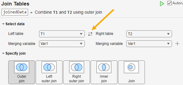
The Join Tables Live Editor task, showing the button for switching the order of the input tables

unique Function: Treat missing values as duplicates

For the unique function, you can treat repeated instances of a missing value as duplicates. For example, unique(A,TreatMissingAsDistinct=false) treats each instance of a missing value in A as a duplicate value.

prctile, quantile, and iqr Functions: Calculate statistics for datetime data

Calculate percentiles, quantiles, or the interquartile range for data in a datetime array using the prctile, quantile, and iqr functions, respectively.

summary Function: Compute enumeration member counts

The summary function now computes the number of occurrences of each member in an enumeration array. If you return a structure that contains the summary, the Members and Counts fields contain this information.

uminus and uplus Functions: Perform unary minus and plus operations directly on tables and timetables

You can now call the uminus and uplus functions directly on tables and timetables without extracting their data. All the variables in your tables and timetables must have data types that these functions support. For more information, see Direct Calculations on Tables and Timetables and Rules for Table and Timetable Mathematics.

 Functionality being removed or changed

mustBeInRange is not recommended

Still runs

The mustBeInRange function is not recommended. Use the mustBeBetween function instead. The mustBeBetween function accepts more data types and uses a simpler way to specify the interval type, using string values identical to those supported by the isbetween function. However, there are no plans to remove mustBeInRange.

This table shows some typical uses of mustBeInRange and how to update your code to use mustBeBetween instead.

Not Recommended

Recommended

mustBeInRange(A,0,100,"inclusive")
mustBeBetween(A,0,100,"closed")
mustBeInRange(A,0,1,"exclusive")
mustBeBetween(A,0,1,"open")
mustBeInRange(A,-5,5,"exclude-lower")
mustBeBetween(A,-5,5,"openleft")

Data Import and Export

 JSON Files: Read and write JSON data as tables and timetables

Read and write JSON files using these functions:

  • readtable and readtimetable — Read JSON data into MATLAB as a table or timetable. You can specify optional name-value arguments to control how readtable and readtimetable treat JSON data.

  • writetable and writetimetable — Write a MATLAB table or timetable to a JSON file. You can specify optional name-value arguments to control how writetable and writetimetable treat JSON data.

When reading JSON data, you can use the detectImportOptions function to detect aspects of the JSON file. When you call detectImportOptions on a JSON file, it returns a JSONImportOptions object that you can use with readtable or readtimetable to customize the import operation.

File Permissions: View and adjust permissions of multiple files using wildcards

You can view the permissions of multiple files by specifying their relative file paths using a wildcard (*) with the filePermissions function. You can then get or set individual permissions of multiple files by using the getPermissions and setPermissions functions, respectively.

FileDatastore Object: Read remote data from a local copy or its source

You can choose whether to read remote data from a local copy or its original source using the CreateLocalCopy name-value argument with fileDatastore. If you set CreateLocalCopy to false, you avoid creating a local copy of your remote data to read from. By default, CreateLocalCopy is true, and fileDatastore downloads remote files before reading them.

delete Function: Remove multiple files by specifying a vector of filenames

With the delete function, you can now remove multiple files by specifying an input vector of filenames.

Comparison Tool: Compare and merge MAT files using improved interface

The Comparison Tool has an improved interface that lets you compare and merge MAT files more efficiently. Improvements include more intuitive merge interactions and new printable reports. For more information, see Compare and Merge MAT Files.

Merge Tool: Resolve conflicts in MAT files using Three-Way Merge tool

If conflicts occur in MAT files during a merge operation, you can now view and resolve the conflicts using the Three-Way Merge tool. For more information, see Resolve Conflicts in MAT Files.

MAT File Comparison: Automate comparison report generation for continuous integration (CI) workflows

You can now programmatically publish comparison reports for MAT files. Automate report generation for continuous integration workflows using the visdiff function.

comparison = visdiff(matFile1,matFile2);
file = publish(comparison);
web(file)

FTP and SFTP: Remove subfolders, nonempty folders, and files using rmdir

Remove subfolders, including nonempty folders, and files from FTP and SFTP servers using the rmdir function with the Recursive name-value argument. Specify Recursive as true to recursively remove the contents of the specified folder. For example:

f = ftp("ftp.example.com")
rmdir(f,"myfolder",Recursive=true)

xmlread Function: Specify XML processing engine for reading XML file

When reading an XML file using the xmlread function, you can specify the XML processing engine as either the MATLAB API for XML Processing (MAXP) or the Java API for XML Processing (JAXP). Specify the XMLEngine name-value argument as "maxp" or "jaxp", respectively.

xmlwrite Function: Specify MAXP DOM object for writing XML file

When writing data to an XML file using the xmlwrite function, you can specify a MATLAB API for XML Processing (MAXP) Document Object Model (DOM) node object as the DOMnode input argument. Previously, the function accepted only a Java API for XML Processing (JAXP) DOM object.

isfilePathInclusive Function: Determine if input is file in current folder, specified location, or MATLAB path

To determine if an input is a file in the current folder, specified location, or MATLAB path, use isfilePathInclusive.

Image Files: imfinfo now returns all EXIF tags associated with HEIF and HEIC images

You can now use imfinfo to get information about all EXIF tags associated with the HEIF or HEIC image files. Previously, imfinfo could return only EXIF orientation tags associated with these images.

This functionality requires MATLAB Support for HEIF/HEIC Image Format, which is available only in the MATLAB desktop environment.

Parallel Processing: Use CFITSIO interface in thread-based environments

You can use the high-level and low-level functions from the CFITSIO interface in thread-based environments, including MATLAB backgroundPool. For a list of high-level and low-level FITS functions, see FITS Files.

Comparison Tool: Compare schemas of HDF5, netCDF, and SOFA files

You can compare the schemas of HDF5, netCDF, and SOFA files by using the Comparison Tool. The tool compares the schemas, but not the data, for these file types. Open the Comparison Tool using the visdiff function.

Scientific File Format Libraries: NetCDF library upgraded to version 4.9.3

The netCDF library is upgraded to version 4.9.3.

Scientific File Format Libraries: CFITSIO library upgraded to version 4.5.0

The CFITSIO library is upgraded to version 4.5.0.

Scientific File Format Libraries: CDF library upgraded to version 3.9.1

The CDF library is upgraded to version 3.9.1.

VideoWriter Function: Support for code generation

The VideoWriter function now supports C/C++ code generation using MATLAB Coder™ for MPEG-4 and AVI profiles.

 Functionality being removed or changed

fileattrib function is not recommended

Still runs

The fileattrib function is not recommended. View and edit file, folder, and symbolic link permissions using the filePermissions function instead. However, there are no plans to remove fileattrib.

H5.open and H5.close functions are not recommended and have no effect

Behavior change

The H5.open and H5.close functions are not recommended and have no effect. Previously, these functions could be used to open and close the HDF5 library in MATLAB. You can still use type-specific functions to open and close HDF5 objects. For example, use the H5F.open and H5F.close functions to open and close an HDF5 file.

disp displays partial content of tall arrays

Behavior change

Starting in R2026a, when you use the disp function to display the content of a tall array, MATLAB displays the top eight rows of data in the tall array. In previous releases, MATLAB displays all the content of the tall array.

For example, this code creates a tall table. In R2025b, MATLAB gathers and displays all the content of the tall table. In R2026a, MATLAB displays only the top eight rows of the tall table.

tt = tall(table(randn(10,1),randn(10,1)));
disp(tt)

Output in R2025bOutput in R2026a
Evaluating tall expression using the Local MATLAB Session:
- Pass 1 of 1: Completed in 0.026 sec
Evaluation completed in 0.033 sec
      Var1        Var2  
    ________    ________

    0.082831      -1.348
     -1.5485     -1.7543
      1.8632    -0.36381
     0.13403    -0.62709
      -1.546     0.44015
     0.43328     -1.5026
     0.10295    -0.20824
    -0.57035     -1.5051
     0.49306      1.8097
    -0.70751     -0.1169
      Var1         Var2  
    _________    ________

      0.87953     0.14766
      -1.4719      1.0809
     -0.27083    -0.05657
    -0.033141     0.17398
      0.53181      1.1838
      0.35187       0.927
      -1.1447     0.65327
      -1.8123     -0.8267
        :           :
        :           :

To re-create the previous behavior, you can gather the tall array into memory and then display the content of the gathered array.

disp(gather(tt))
Alternatively, you can avoid a computationally expensive gather operation by displaying the output of the tall array without using a semicolon. This will show the top eight rows of data in the tall array.

Mathematics

ode Object: Calculate Jacobians using automatic differentiation

You can use the JacobianMethod property of an ode object to specify whether the solver calculates the Jacobians for a given problem using finite differences or automatic differentiation. By default, the Jacobians are calculated using finite differences. The automatic differentiation method might be faster for large stiff systems and more accurate for sensitivity analyses.

ode Object: Solve implicit ODEs using IDAS solver

You can now solve implicit ODEs using the IDAS solver by specifying the Solver property of a fully implicit ode object as "idas".

Integral Functions: Integrate functions with scalar inputs

You can integrate functions written for scalar inputs when using the integral, integral2, and integral3 functions by specifying the Vectorized name-value argument as false.

MATLAB Support Package for Quantum Computing: Parameterize circuits in local simulation (July 2026)

You can create parameterized rotation gates by specifying the rotation or phase angle as a parameterized expression using a string scalar, string vector, symbolic scalar, or symbolic vector in these creation functions:

Quantum circuits now have a Parameters property that lists the parameters used by circuit gates. If a circuit has parameterized gates, you can specify parameter values when calling the simulate, getMatrix, and observe functions on the circuit.

 Functionality being removed or changed

Combining exponentiation operators with unary operators or logical negations without parentheses will not be supported in a future release

Still runs

When you specify a sequence of exponentiation operators combined with unary operators or logical negations in the exponents, you will have to use parentheses to explicitly specify the order of operations. Omitting parentheses in operations that include ^-, .^-, ^+, .^+, ^~, or .^~ when chained with other exponentiation operators will result in an error in a future release.

For example, the result of an operation such as y = 4^-3^-2 depends on the order in which exponentiation and negation are performed. For this reason, use parentheses to explicitly specify the intended order of operations. For example:

y = (4^(-3))^(-2)
y =
    4096
y = 4^(-(3^(-2)))
y =
    0.8572
y = 4^((-3)^(-2))
y =
    1.1665

conv function returns row vector for full convolution unless both input vectors are column vectors

Behavior change

For the conv function, when you compute a full convolution using w = conv(u,v) or w = conv(u,v,"full"), the output w is a row vector unless both input vectors u and v are column vectors.

For example, if you convolve a row vector and a column vector, the output is a row vector.

u = [1 0 1];
v = [2; 7; 4];
w = conv(u,v)
w =
     2     7     6     7     4
If you convolve two column vectors, the output is a column vector.
u = [1; 0; 1];
v = [2; 7; 4];
w = conv(u,v)
w =
     2
     7
     6
     7
     4

In previous releases, when computing a full convolution, the conv function returned either a row or column vector depending on the orientations and lengths of u and v.

For example, in previous releases, conv returned the full convolution of a 1-by-3 row vector and a 3-by-1 column vector as a 5-by-1 column vector.

u = [1 0 1];
v = [2; 7; 4];
w = conv(u,v)
w =
     2
     7
     6
     7
     4
However, conv returned the full convolution of a 1-by-3 row vector and a 2-by-1 column vector as a 1-by-4 row vector.
u = [1 0 1];
v = [2; 7];
w = conv(u,v)
w =
     2     7     2     7

There are no changes to the output of w = conv(u,v,"same") or w = conv(u,v,"valid"), where the output still follows the orientation of the first input vector u.

cast, double, single, int8, int16, int32, int64, uint8, uint16, uint32, and uint64 functions preserve complexity when converted complex input has zero imaginary part

Behavior change

The cast, double, single, int8, int16, int32, int64, uint8, uint16, uint32, and uint64 functions preserve complexity when converting a complex input, even if the converted result has a zero imaginary part.

For example, convert a complex number of type double to type single. The output is a complex number of type single with a zero imaginary part.

a = complex(1,1e-48);
b = cast(a,"single")
b =

  single
   1.0000 + 0.0000i
whos
  Name             Size            Bytes  Class     Attributes

  a                1x1                16  double    complex   
  b                1x1                 8  single    complex   
Checking whether the converted number is real returns a logical 0.
tf = isreal(b)
tf =

  logical
   0

For comparison, in previous releases, converting the same number returned a real number of type single.

a = complex(1,1e-48);
b = cast(a,"single")
b =

  single
     1
whos
  Name             Size            Bytes  Class     Attributes

  a                1x1                16  double     complex   
  b                1x1                 4  single               
Checking whether the converted number was real returned a logical 1 instead.
tf = isreal(b)
tf =

  logical
   1

pow2 and log2 functions no longer accept complex inputs when you specify two inputs or two outputs

Errors

The pow2 and log2 functions return an error if you specify complex inputs when using the two-input or two-output syntax. These syntaxes no longer accept complex inputs. In previous releases, the two-input syntax of pow2 and the two-output syntax of log2 ignored the imaginary parts of complex inputs and processed only the real parts.

To preserve the behavior of previous releases, use the real function to extract the real parts of complex inputs, as shown in this table.

Not Recommended (Errors)Recommended
X = 2 + 1i;
E = 2i;
Y = pow2(X,E);
X = 2 + 1i;
E = 2i;
Y = pow2(real(X),real(E));
X = 2 - 1i;
[F,E] = log2(X);
X = 2 - 1i;
[F,E] = log2(real(X));

pol2cart and sph2cart functions no longer accept complex inputs

Errors

The pol2cart and sph2cart functions return an error for complex inputs. These functions no longer accept complex inputs because their inverse functions, cart2pol and cart2sph, do not accept complex inputs.

To preserve the behavior of previous releases for complex inputs, use the formulas that map polar, cylindrical, or spherical coordinates to Cartesian coordinates, as shown in this table.

Not Recommended (Errors)Recommended
theta = 2i;
rho = 1i;
[x,y] = pol2cart(theta,rho);
theta = 2i;
rho = 1i;
x = rho*cos(theta);
y = rho*sin(theta);
azimuth = 1i;
elevation = 2i;
r = 1;
[x,y,z] = sph2cart(azimuth,elevation,r);
azimuth = 1i;
elevation = 2i;
r = 1;
x = r*cos(elevation)*cos(azimuth);
y = r*cos(elevation)*sin(azimuth);
z = r*sin(elevation);

Graphics

 Web Canvas: Create webpages with interactive graphics

Create HTML files containing interactive web canvases directly from your MATLAB plots and live scripts. A web canvas is an interactive plot element within an HTML page. Most visualizations in a web canvas support pan, zoom, and rotate interactions.

You can open an HTML file containing a web canvas using a web browser with an internet connection, share the file with others, or host it on a web server. No MATLAB license is required to view and interact with graphics in a web canvas. For more information, see Display Interactive Graphics on Webpages.
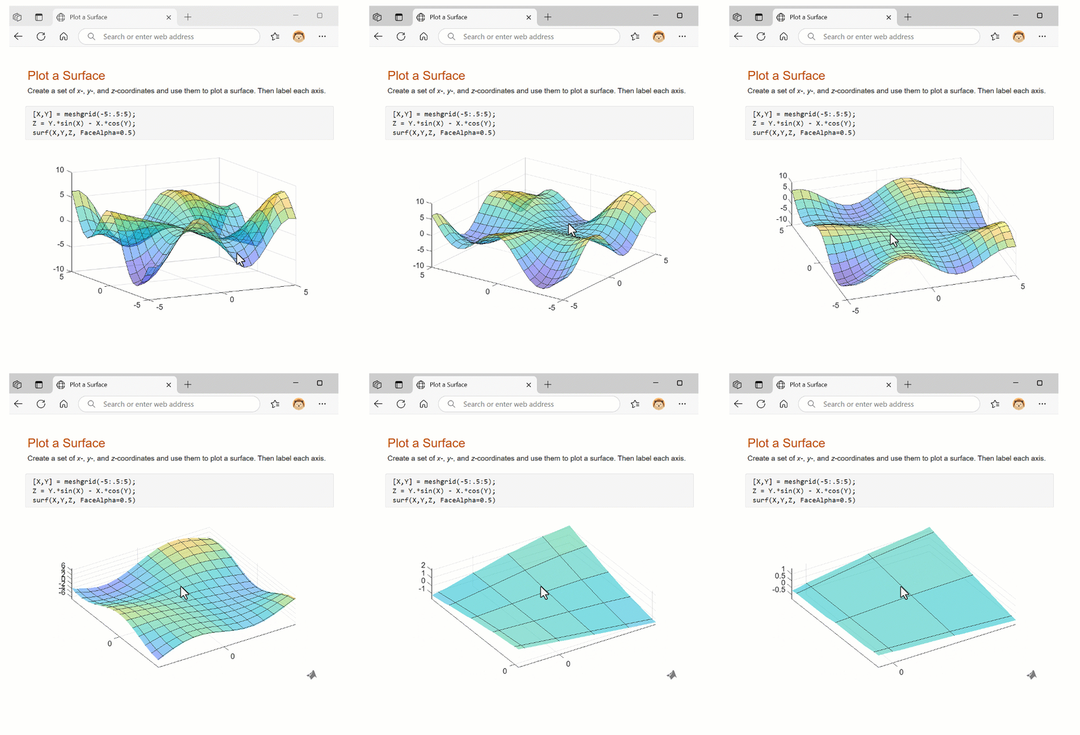
Webpage displaying the contents of a live script, including an interactive web canvas.

 raincloudplot Function: Visualize grouped numeric data by using rain cloud plots

To create rain cloud plots for grouped numeric data, use the raincloudplot function. The upper half of each rain cloud plot displays a violin plot, and the lower half displays a swarm chart. If you specify a matrix of input data, raincloudplot creates a separate plot for each column in the matrix. You can also specify a positional grouping variable to split your data into groups.
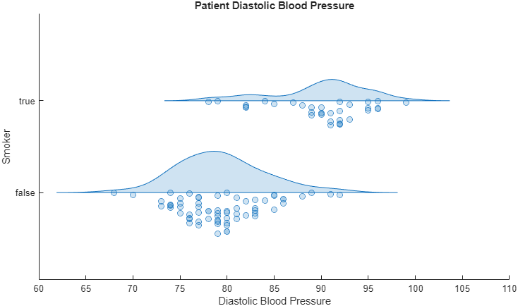
Rain cloud plot that shows distributions of diastolic blood pressure for smokers and nonsmokers

Plotting Table Data: Create plots by passing tables directly to plotting functions

These plotting functions now accept tables, timetables, and table variables as input arguments: bar, barh, area, histogram, polarhistogram, geodensityplot, and binscatter. In most cases, the axis labels and the legend (if present) automatically display the table variable names.

Axes Toolbar: Interact with axes content using improved interface

The axes toolbar has an improved interface for interacting with axes content.

  • The toolbar appears persistently on axes. You can expand and collapse the toolbar by clicking a button. Previously, the toolbar appeared only when you hovered your mouse over the axes.

  • The appearance of the toolbar automatically matches the theme of the figure.

  • The toolbar is keyboard accessible and compatible with touchscreens and screen readers.

  • The toolbar supports SVG files for button icons and uses them by default. Previously, the only file types that the toolbar supported for icons were PNG, JPEG, and GIF. SVG icons allow for a sharper appearance than PNG and JPEG icons.

Additionally, the toolbar has a new property named Expanded. Specify Expanded as "off" (the default) to collapse the toolbar, and as "on" to expand the toolbar..

Axes Toolbar: Specify location of toolbar relative to axes

Specify the location of the axes toolbar relative to the axes by using the ToolbarLocation property of the axes object. By default, MATLAB® automatically selects the toolbar location based on the current view.

Axes Toolbar: Display or hide axes toolbar in standalone visualizations

Display or hide the axes toolbar in pie charts, donut charts, scatter histograms, parallel plots, bubble clouds, and heatmap charts by setting the ToolbarVisible property of the chart. The axes toolbar is visible in these charts by default, but you can hide it by setting the property to "off".

Axes Toolbar: Specify tooltip text for toolbar drop-down menus

When you create a custom drop-down menu for the axes toolbar using a ToolbarDropdown object, you can specify tooltip text for the menu button by setting its Tooltip property. The tooltip text appears when you hover the pointer over the button.

imresize Function: Apply padding that replicates border pixels

The imresize function now supports padding that replicates the pixel values at the border of the image. To apply padding that replicates border pixel values, specify the new Padding name-value argument as "replicate". By default, or if you specify the Padding name-value argument as "symmetric", the imresize function applies symmetric padding.

Stability and Memory Usage: Create graphics with improved stability and memory usage

Scatter plots, surface plots, pseudocolor plots, and images have improved stability and memory usage. As a result, you can create more of these visualizations from large data sets than in the previous release without experiencing crashes or system resource issues.

 Functionality being removed or changed

opengl function has been removed

Errors

The opengl function has been removed. To query the graphics renderer, use the rendererinfo function instead.

In R2025a, MATLAB stopped using OpenGL® technology to render graphics, so you no longer need to set the renderer in your graphics workflows.

Links are preserved across multiple calls to the linkaxes function

Behavior change

Calls to the linkaxes function preserve links established by prior calls to the function. Previously, calls to the linkaxes function canceled links established by prior calls to the function.

For example, link the x-axes of ax1 and ax2 and then link the y-axes of ax1 and ax3.

linkaxes([ax1 ax2],"x")
linkaxes([ax1 ax3],"y")
Starting in R2026a, the second function call preserves the link between the x-axes of ax1 and ax2. In previous releases, the second function call canceled the link between the x-axes of ax1 and ax2.

To preserve the previous behavior, you can explicitly cancel prior links before creating a new link. For example, to cancel all links involving ax1 or ax2, call linkaxes([ax1 ax2],"off").

PickableParts property of Axes objects is "all" by default

Behavior change

Starting in R2026a, the default value for the PickableParts property of Axes, UIAxes, PolarAxes, and GeographicAxes objects is "all". Previously, the default value was "visible".

Figure Copy settings use consistent default figure sizes on all systems

Behavior change

In the MATLAB Figure Copy Settings window, if you clear the Match on-screen size check box with no other changes, or if you make other changes and click Restore Defaults, the default size of the copied figure is consistently 1000-by-600 pixels regardless of the display resolution.

Previously, if you changed the settings in these ways, the default size of the copied figure depended on the resolution of the system display, which often resulted in inconsistent image sizes.

imshow function always sets InitialMagnification to "fit" in the Live Editor

Behavior change

When you use the imshow function in the Live Editor, the default value of the InitialMagnification name-value argument is now "fit". Previously, the default value was 100, and titles might have appeared cropped.

You do not need to update your code. If you specify InitialMagnification in a live script, the function ignores it without error. However, image sizes might differ from previous releases.

Marginal histograms of scatterhistogram plots update after interaction is complete

Behavior change

If you create a scatterhistogram plot and then pan or zoom in a way that affects the shape of the marginal histograms, the histograms update after you lift your finger from your device or mouse.

Previously, the marginal histograms updated as you performed the interaction (before lifting your finger).

ButtonDownFcn property of AxesToolbar, ToolbarStateButton, ToolbarPushButton, and ToolbarDropdown objects has been removed

Errors

The ButtonDownFcn property of AxesToolbar, ToolbarStateButton, ToolbarPushButton, and ToolbarDropdown objects has been removed. Previously, these objects each had a ButtonDownFcn property, but the property had no effect.

Children property of ToolbarStateButton and ToolbarPushButton objects has been removed

Errors

The Children property of ToolbarStateButton and ToolbarPushButton objects has been removed. Previously, these objects each had a Children property, but the property had no effect.

App Building

UI Components: Associate label with component

Associate a label with the UI component that it describes by using the Label property of the component. Screen readers use the label text to describe the component when an app user navigates through your app.

For more information, refer to the object page of the labeled UI component. For example, see the Label property of the edit field component.

App Designer: Share app in MATLAB Drive from App Designer

You can share an app that you have stored in MATLAB Drive directly from App Designer.

With the app open in App Designer, on the Designer tab, in the Share section, select Share > MATLAB Drive. To manage permissions, select Invite Members and then add members with read or edit permissions to your app folder. To share your app with others through a link, select Create Link.

For more information, see Share App in MATLAB Drive.

App Designer: View code details in Code View using status bar

When you have an app open in Code View, you can view details about your app code in the status bar at the bottom of App Designer. For example, you can view how many times a highlighted variable appears in your code or the name of the function your cursor is in.
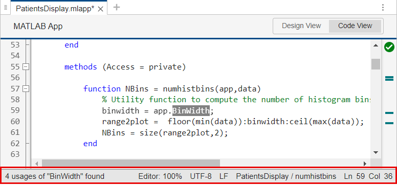
App Designer app open in Code View. The status bar at the bottom of the app shows information such as the number of usages of the highlighted text, the name of the function the cursor is in, and the line number of the cursor.

App Designer: Update app layout and navigate code more easily

In Design View, when you move UI components on the canvas, you can constrain vertical or horizontal movement by holding Shift while you drag. For example, to move a button to the right without moving it up or down, hold Shift and then drag the button.

You can also reorder labeled components and other groups of components together. For example, to bring a component and its associated label to the front, select the component and its label, and then on the Canvas tab of the toolstrip, in the Arrange section, select Reorder > Bring to Front.

Finally, in Code View, in the Code Browser panel, when you select the name of a callback, function, or property, App Designer scrolls that element into view and highlights it in your code.

App Designer: Use custom keyboard shortcuts in Code View

Custom keyboard shortcuts that you specify for MATLAB now apply in App Designer Code View. You can use Emacs keyboard shortcuts or define your own custom shortcuts.

To change your keyboard shortcuts, in MATLAB, on the Home tab, in the Environment section, click Settings. Then, select Keyboard > Shortcuts. For more information, see Customize Keyboard Shortcuts.

App Designer: Remove Simulink dependency from app

For an app originally created as a blank app from the App Designer start page, App Designer now automatically removes all Simulink dependencies whenever the app does not contain any Simulink functionality. For example, if you create a blank app, add a Simulink UI component, and then delete that Simulink UI component, App Designer removes the dependency on Simulink from that app.

 Functionality being removed or changed

Interactions with app toolbar buttons have different keyboard shortcuts

Still runs

Interactions with buttons on an app toolbar have different keyboard shortcuts. The new shortcuts apply to push tool and toggle tool UI components and to buttons on an axes toolbar. These keyboard shortcuts are more consistent with keyboard shortcuts for other UI components in apps.

To move focus to a button on an app toolbar, use the Tab key. Once a button is in focus, use the arrow keys to navigate between different buttons on the toolbar.

In previous releases, the Tab key navigated between different buttons.

Performance

MATLAB Startup: Improved performance

MATLAB starts up faster in R2026a than in R2024b and previous releases. This improvement is most noticeable after the first startup and when starting MATLAB with multiple files open in the Editor.

For example, after the first startup, MATLAB R2026a starts up about 1.3x times faster than R2024b.

The approximate startup times are:

R2024b: 9.12 s

R2026a: 7.25 s

When starting with 15 code files previously open in the Editor, MATLAB R2026a starts about 1.4x times faster than R2024b.

The approximate startup times are:

R2024b: 11.24 s

R2026a: 8.22 s

Startup was timed on a Windows 11, Intel Xeon 6-Core Processor @ 3.60 GHz test system by measuring the interval between launching MATLAB and the Command Window being ready to accept commands.

If your startup time is significantly slower than these approximate times, configuration issues or other factors might be affecting your MATLAB startup. For troubleshooting steps, see Resolve Slow Startup.

 power Function: Improved performance when computing element-wise powers with integer exponents

The power function (.^) shows improved performance when computing element-wise powers with integer exponents. For example, this code raises every element in a 5000-by-5000 array to the power of 3. The code is about 3.8x faster than in the previous release.

function t = timingPower
x = rand(5000);
y = @() x.^3;
t = timeit(y);
end

The approximate execution times are:

R2025b: 0.80 s

R2026a: 0.21 s

The code was timed on a Windows 11, AMD EPYC 74F3 24-Core Processor @ 3.19 GHz test system by calling the timingPower function.

 Compatibility Considerations

This performance improvement arises from code changes that also result in slightly different round-off behavior in double precision, leading to more accurate results. For example, this code now returns a result that is more accurate to the 15th digit after the decimal point in long scientific notation.

format longE
y = 0.4543.^3
y =
     9.376229100700000e-02

Previously, the same code returned this result.

format longE
y = 0.4543.^3
y =
     9.376229100699998e-02

Note that MATLAB converts a decimal number input, like 0.4543, to the nearest representable double-precision binary value, which might not be exactly equal to the original decimal input. For this reason, although the .^ operator is now more accurate in double precision, the result might differ from a calculation performed using the exact representation of the operands.

 log Function: Improved performance when computing natural logarithms in double precision

The log function shows improved performance when computing natural logarithms in double precision. For example, this code computes the natural logarithms of 100,000,000 real numbers within the interval of 0 to 1000. The code is about 2.8x faster than in the previous release.

function t = timingLog
x = rand(1,1e8)*1000;
y = @() log(x);
t = timeit(y);
end

The approximate execution times are:

R2025b: 0.79 s

R2026a: 0.28 s

The code was timed on a Windows 11, AMD EPYC 74F3 24-Core Processor @ 3.19 GHz test system by calling the timingLog function.

 Compatibility Considerations

This performance improvement arises from code changes that also result in slightly different round-off behavior in double precision, leading to more accurate results. For example, this code now returns a result that is more accurate to the 15th digit after the decimal point in long scientific notation.

format longE
Y = log(1.63340913276288)
Y =
     4.906693231856701e-01

Previously, the same code returned this result.

format longE
Y = log(1.63340913276288)
Y =
     4.906693231856700e-01

Note that MATLAB converts a decimal number input, like 1.63340913276288, to the nearest representable double-precision binary value, which might not be exactly equal to the original decimal input. For this reason, although the log function is now more accurate in double precision, the result might differ from a calculation performed using the exact representation of the input.

duration Data Type: Improved performance with duration arrays

Operations on duration arrays show improved performance. These operations include but are not limited to:

  • Arithmetic operations

  • Array creation

  • Array indexing

  • Concatenation

  • Reshaping

  • Sorting

For example, this code creates a duration scalar. The code is about 108x faster than in the previous release.

function timingTest
for i = 1:1e6
    d = duration(0,0,30);
end
end

The approximate execution times are:

R2025b: 12.93 s

R2026a: 0.12 s

As another example, this code assigns an element to a duration array. The code is about 28x faster than in the previous release.

function timingTest
s = seconds(1:1e6);
for i = 1:1e6
    s(1) = 0;
end
end

The approximate execution times are:

R2025b: 0.57 s

R2026a: 0.02 s

The code was timed on a Windows 11, AMD EPYC 74F3 24-Core Processor @ 3.19 GHz test system using the timeit function.

timeit(@timingTest)

filter Function: Improved performance for finite impulse response (FIR) filters

The filter function shows improved performance for FIR filters. FIR filters are characterized by a finite impulse response duration and a rational transfer function in the z-domain that has only zeros and no poles. The performance improvement is most noticeable when the transfer function has a significant number of coefficients.

For example, this code filters an input signal of length 1,000,000 using a low-pass filter with 10,001 coefficients in the numerator of the transfer function. The code is about 2.3x faster than in the previous release.

function ts = timingFilter
t = 1:1000000;
x = sin(5e-5*t) + sin(10*t) + 0.1*rand(size(t));

N = 10000;
freq = 0.5;
k = -(N/2):(N/2);
h_ideal = sin(freq*pi*k)./(pi*k);
h_ideal(k==0) = freq;
w = 0.54 - 0.46*cos(2*pi*(0:N)/N);
b = h_ideal.*w;

y = @() filter(b,1,x);
ts = timeit(y);
end

The approximate execution times are:

R2025b: 0.28 s

R2026a: 0.12 s

The code was timed on a Windows 11, AMD EPYC 74F3 24-Core Processor @ 3.19 GHz test system by calling the timingFilter function.

nufft and nufftn Functions: Improved performance with nonuniform sample points and query points

The nufft and nufftn functions show improved performance when operating on nonuniformly spaced sample points and query points. These functions achieve a significant performance increase by using more efficient interpolation algorithms.

For example, this code computes the 1-D nonuniform discrete Fourier transform of a 10,000-by-1 array using 10,000 nonuniform sample points and 10,000 nonuniform query points. The code is about 330x faster than in the previous release.

function t = timing_nufft
n = 10000;
x = randn(n,1);
t = rand(n,1);
f = 10000*rand(n,1);

y = @() nufft(x,t,f);
t = timeit(y);
end

The approximate execution times are:

R2025b: 1.65 s

R2026a: 0.005 s

As another example, this code computes the 2-D nonuniform discrete Fourier transform along each dimension of a 100-by-100 array using 10,000-by-2 nonuniform sample points and 10,000-by-2 nonuniform query points. The code is about 123x faster than in the previous release.

function t = timing_nufftn
n = 100;
x = randn(n,n);
t = rand(n^2,2);
f = 100*rand(n^2,2);
  
y = @() nufftn(x,t,f);
t = timeit(y);
end

The approximate execution times are:

R2025b: 1.72 s

R2026a: 0.014 s

The code was timed on a Windows 11, AMD EPYC 74F3 24-Core Processor @ 3.19 GHz test system by calling the timing_nufft and timing_nufftn functions.

kde Function: Improved performance of kernel density estimate computations

The kde function shows improved performance. The performance improvement depends on the size of the univariate data set, the number of evaluation points, and the bandwidth for the kernel smoothing function. For example, the kernel density estimate computation in this code is about 15x faster than in the previous release.

function timingTest
data = randn(1e5,1);
[f,xf,bw] = kde(data,NumPoints=1e4);
end

The approximate execution times are:

R2025b: 11 s

R2026a: 0.72 s

The code was timed on a Windows 11, Intel Xeon CPU W-2133 @ 3.60 GHz test system using the timeit function.

timeit(@timingTest)

join Function: Improved performance with tall tables when returning two outputs

The join function shows improved performance when the first input is a tall table and two output arguments are returned. The second input argument can be either an in-memory table or the result of a reduction operation on a tall table. The improvement is a result of reducing the number of reads or passes through the tall table.

For example, this code joins a tall table and an in-memory table and gathers both the joined table and the index vector. The code is about 5.3x faster than in the previous release.

function t = timeJoinWithTwoOutputs
% Run tall code on the local MATLAB session
mapreducer(0)

% Create sample data
keysVar = (1:5e3)';
keysVarShuffled = randi(5e3,1e4,1);
x = randi(1e5,1e4,1);
y = randi(10,5e3,1);
z = randi(1e3,5e3,1,"single");
zz = randi(1e3,1e4,1,"single");

% Create tall table
t = table(x,keysVarShuffled,zz,VariableNames=["X","keys","ZZ"]);
tallTable = tall(t);

% Create in-memory table
inMemoryTable = table(y,z,keysVar,VariableNames=["Y","Z","keys"]);

% Measure time for join
    function joinWithTwoOutputs
        [C,idxb] = join(tallTable,inMemoryTable);
        gather(C,idxb);
    end
t = timeit(@joinWithTwoOutputs);
end

The approximate execution times are:

R2025b: 0.74 s

R2026a: 0.14 s

The code was timed on a Windows 11, Intel Xeon Silver CPU 4310 @ 2.1 GHz test system by calling the timeJoinWithTwoOutputs function.

innerjoin Function: Improved performance when joining tall and in-memory tables

The innerjoin function shows improved performance when the first input is a tall table. The second input argument can be either an in-memory table or the result of a reduction operation on a tall table. The improvement is a result of reducing the number of reads or passes through the tall table.

For example, this code performs an inner join of a tall table and an in-memory table and gathers the joined table into memory. The code is about 5.9x faster than in the previous release.

function t = timeInnerJoinWithTall
% Run tall code on the local MATLAB session
mapreducer(0);

% Create tall table
x = randi(1e3,1e4,1);
y = randi(1e3,1e4,1);
t = table((1:length(x))',x,y,VariableNames=["keys","Var1","Var2"]);
tallTable = tall(t);

% Create in-memory table
inMemoryTable = table(randperm(1e4,100)',x(1:100),y(1:100), ...
                VariableNames=["keys","Var3","Var4"]);
 
% Measure time for innerjoin 
    function timeInnerJoin 
        C = innerjoin(tallTable,inMemoryTable); 
        gather(C); 
    end 
t = timeit(@timeInnerJoin); 
end

The approximate execution times are:

R2025b: 1.58 s

R2026a: 0.27 s

The code was timed on a Windows 11, Intel Xeon Silver CPU 4310 @ 2.1 GHz test system by calling the timeInnerJoinWithTall function.

Data Grouping Functions: Improved performance for numeric or string grouping vector

These functions show improved performance when the grouping variable or vector type is numeric or string:

When the grouping variable or vector is numeric, the improvement is most noticeable when the total number of elements and the number of elements per group are large.

For example, this code computes the group-wise mean for 12,500,000 elements split into 25 numeric groups. The code is about 9x faster than in the previous release.

function t = timingNumeric
numberOfGroups = 25;
elementsPerGroup = 5e5;
groups = repmat(1:numberOfGroups,1,elementsPerGroup)';
data = randn(numel(groups),1);
G = @() groupsummary(data,groups,"mean");
t = timeit(G);
end

The approximate execution times are:

R2025b: 1.35 s

R2026a: 0.15 s

When the grouping variable or vector type is string, the improvement is most noticeable when the total number of elements is large and the number of elements per group is small.

For example, this code computes the group-wise mean for 5,000,000 elements split into 50 string groups. The code is about 4.3x faster than in the previous release.

function t = timingString
numberOfGroups = 50;
elementsPerGroup = 1e5;
groups = repmat(string(1:numberOfGroups),1,elementsPerGroup)';
data = randn(numel(groups),1);
G = @() groupsummary(data,groups,"mean");
t = timeit(G);
end

The approximate execution times are:

R2025b: 1.03 s

R2026a: 0.24 s

The code was timed on a Windows 11, AMD EPYC 74F3 24-Core Processor @ 3.19 GHz test system by calling the timingNumeric and timingString functions.

sort and sortrows Functions: Improved performance for 8-bit and 16-bit integer data

The sort and sortrows functions show improved performance when sorting elements of type int8, uint8, int16, or uint16. The improvement is most noticeable when the number of elements to sort is large.

For example, this code sorts a 100,000,000-element column vector of type int8. The code is about 5.0x faster than in the previous release.

function t = timingTest
A = randi(intmax("int8"),[1e8 1],"int8");
S = @() sort(A);
t = timeit(S);
end

The approximate execution times are:

R2025b: 1.06 s

R2026a: 0.21 s

The code was timed on a Windows 11, AMD EPYC 74F3 24-Core Processor @ 3.19 GHz test system by calling the timingTest function.

readlines Function: Improved performance when reading lines of a file as string arrays

The readlines function shows improved performance when reading lines of data from a file as string arrays. For example, this code creates a 48MB test file, reads the lines of data from the file, and then deletes the file. The call to readlines is about 2.9x faster than in the previous release.

function readlinesPerformance
%% Create the test file.
rng(1)
lines = 1e6;
lineLength = randi([30 70],[1 lines],"uint8");
fid = fopen("testfile.txt","W");
for ii = 1:numel(lineLength)
    data = randi([33 127],[1 lineLength(ii)],"uint8");
    fwrite(fid,[data 10],"uint8");
end
fclose(fid);

%% Timing test for readlines
f = @() readlines("testfile.txt");
t = timeit(f)

%% Delete test file.
delete testfile.txt;
end

The approximate execution times are:

R2025b: 0.85 s

R2026a: 0.29 s

The code was timed on a Windows 11, AMD EPYC 74F3 24-Core Processor @ 3.19 GHz test system by calling the readlinesPerformance function.

mget Function: Improved performance when downloading files from SFTP and FTP servers

The mget function shows improved performance when downloading files from SFTP and FTP servers. For example, this code connects to an FTP server, downloads a test file from the server into a local folder, and then deletes the local folder and test file. The call to mget is about 1.6x faster than in the previous release.

function mgetPerformance
f = ftp("ftp.ngdc.noaa.gov/geomag/wmm/");
m = @()mget(f,"wmm2015v2/shapefiles/2019_WMM2015v2_DI_shape_geographic.zip","localTestFolder");
t = timeit(m)
rmdir localTestFolder s
end

The approximate execution times are:

R2025b: 5.99 s

R2026a: 3.74 s

The code was timed on a Windows 11, AMD EPYC 74F3 24-Core Processor @ 3.19 GHz by calling the mgetPerformance function.

ftp Function: Improved performance when connecting to subfolders

The ftp function shows improved performance when connecting to subfolders. For example, this code connects to a subfolder on an FTP server. The call to ftp is about 2x faster than in the previous release.

function timingTest
ftp("ftp.ngdc.noaa.gov/pub/outgoing/mgg/nos/H13873/H13873/Raw/Positioning/FA_S220_EM712/2024-129/129_B");
end

The approximate execution times are:

R2025b: 0.94 s

R2026a: 0.48 s

The code was timed on a Windows 11, AMD EPYC 74F3 24-Core Processor @ 3.19 GHz using the timeit function.

timeit(@timingTest)

Line Plot Interactions: Improved responsiveness for panning and zooming

Line plots created using the plot function show improved responsiveness for panning and zooming. If you plot approximately 2.5 million or more points and then pan or zoom within the axes, the content that was previously outside the boundaries of the axes comes into view more quickly in R2026a than in the previous release. Before R2026a, gaps in the content appeared as you panned or zoomed.

For example, on a Windows 11, AMD EPYC 74F3 24-Core Processor @ 3.19 GHz test system that has an NVIDIA® A16-2B GPU with 2 GB RAM, if you run this code and then pan within the axes, the content updates immediately without any gaps.

x = 1:2500000;
y = [log(x') log(x')+2 log(x')+4] + rand(2500000,1);
plot(x,y)
xlim([1500 4500])
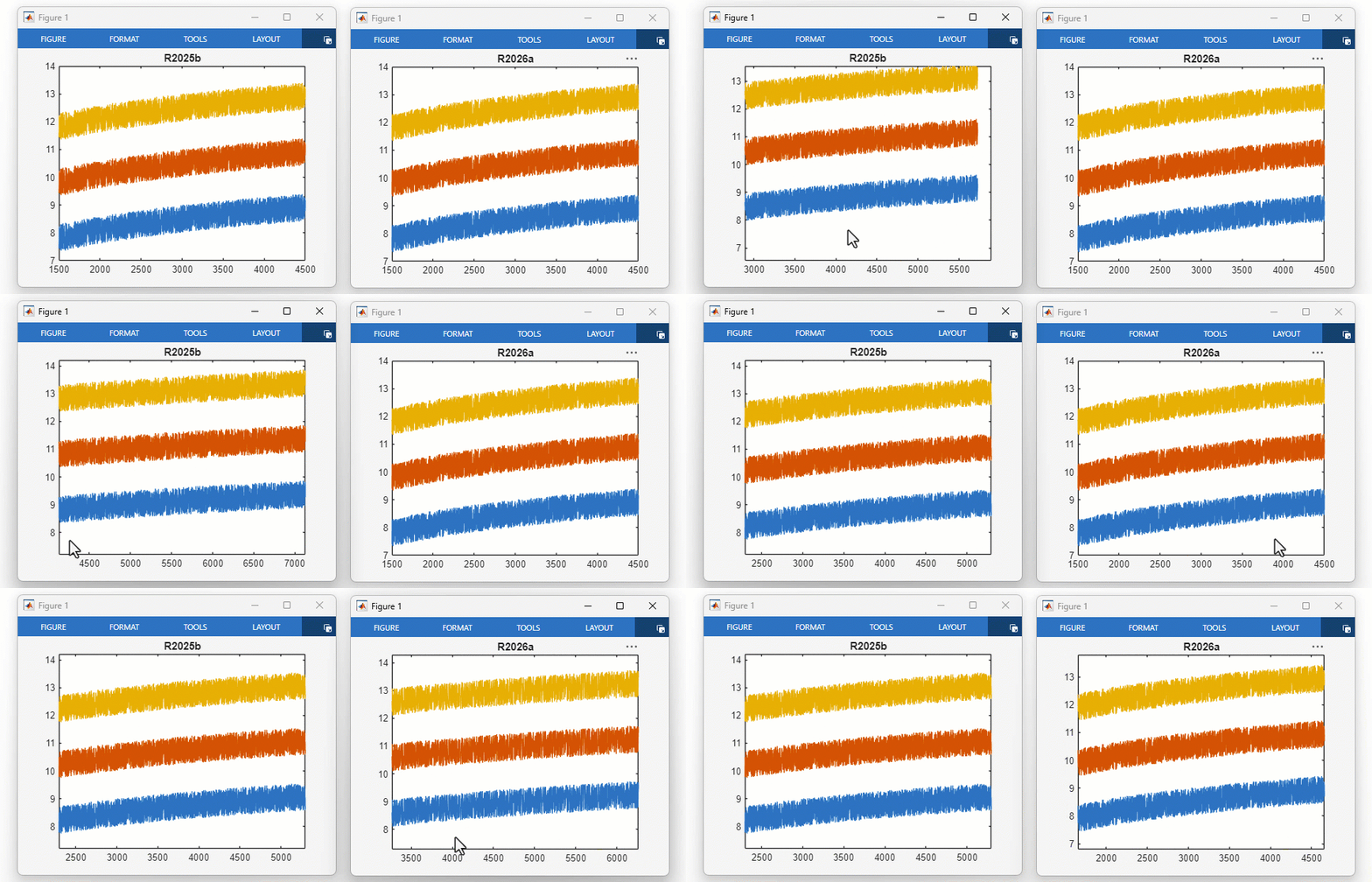
Animation of panning within a line plot in R2025b and R2026a

Quiver and Stem Plot Interactions: Improved responsiveness for panning and zooming

quiver and stem plots show improved responsiveness for panning and zooming. This improvement is more noticeable when you plot approximately 25,000 or more points.

For example, on a Windows 11, AMD EPYC 74F3 24-Core Processor @ 3.19 GHz test system that has an NVIDIA A16-2B GPU with 2 GB RAM, if you run this code and then pan within the axes, the panning action is smoother and follows the cursor more closely in R2026a than in the previous release.

[x1,y1] = meshgrid(0:1:150, 0:1:300);
[x2,y2] = meshgrid(151:1:300, 0:1:300);
u1 = cos(x1);  
v1 = sin(y1);  
quiver(x1,y1,u1,v1,LineWidth=2)
hold on
u2 = cos(x2);  
v2 = sin(y2);
quiver(x2,y2,u2,v2,LineWidth=2)
xlim([130 170])
ylim([130 170])
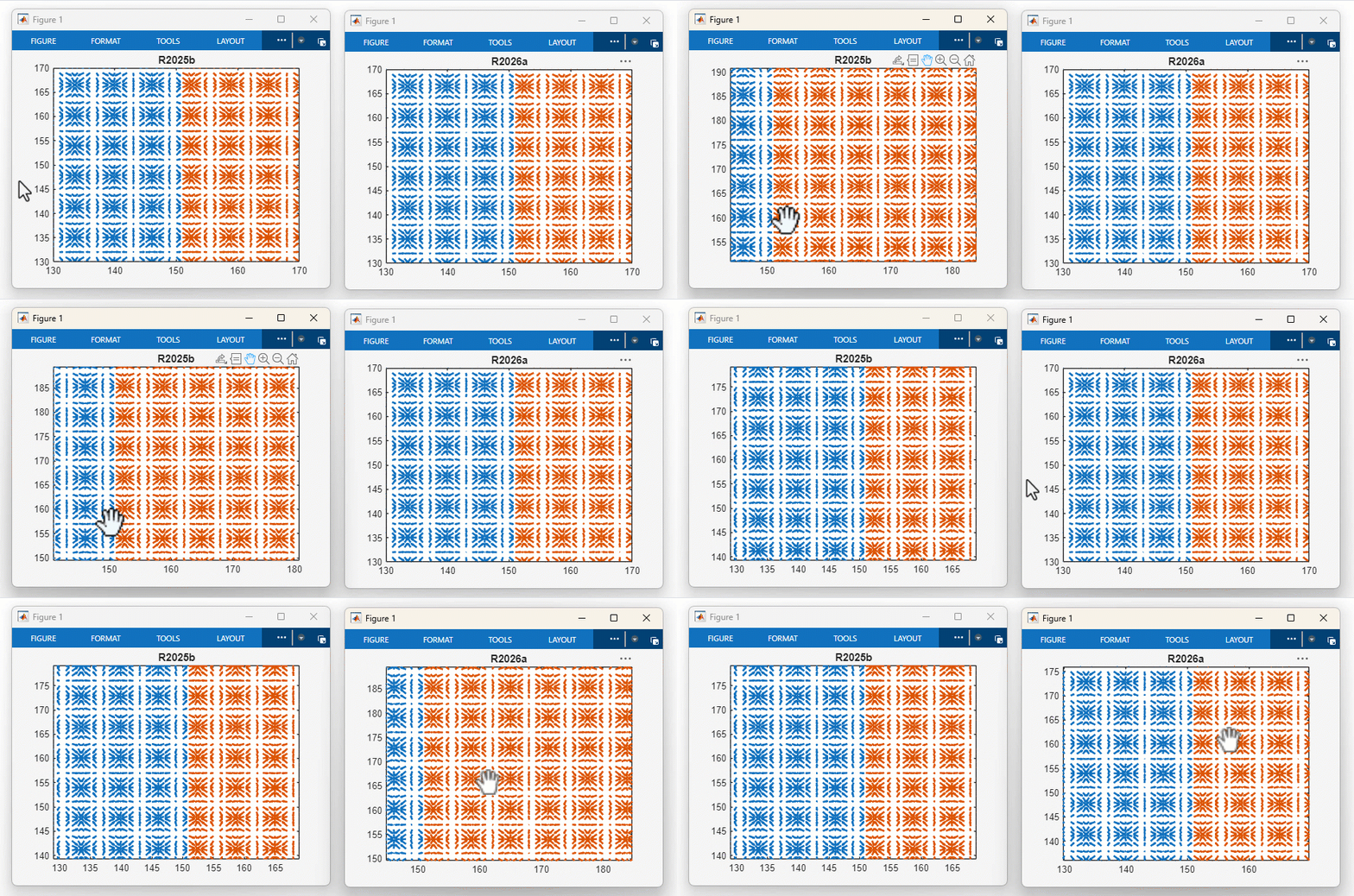
Animation of panning within a quiver plot in R2025b and R2026a

Scatter Histogram Interactions: Improved responsiveness for panning and zooming

Scatter histogram plots show improved responsiveness for panning and zooming. If you plot a large number of points using the scatterhistogram function, the interaction is smoother and the visual changes follow the cursor more closely.

For example, on a Windows 11, AMD EPYC 74F3 24-Core Processor @ 3.19 GHz test system that has an NVIDIA A16-2B GPU with 2 GB RAM, if you run this code and then pan within the plot, the panning action follows the cursor more closely in R2026a than in the previous release.

x1 = 2*randn(50000,1) - 1; 
x2 = randn(50000,1) + 10; 
y1 = 2*randn(50000,1) - 1; 
y2 = randn(50000,1) + 7;
x = [x1; x2]; 
y = [y1; y2];
g = [ones(50000,1); ones(50000,1)*2];
scatterhistogram(x,y,GroupData=g,MarkerAlpha=0.2)
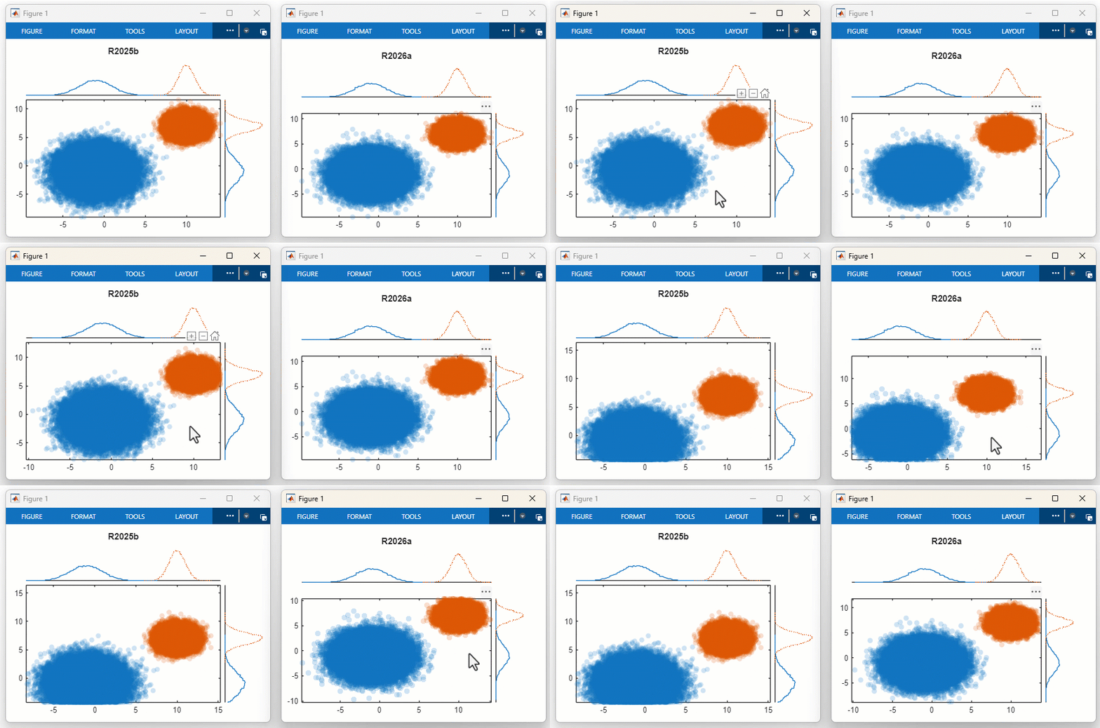
Animation of panning within a scatterhistogram plot in R2025b and R2026a

validatecolor and fliplightness Functions: Improved performance for validating and flipping colors

The validatecolor function shows improved performance, and this improvement positively impacts the performance of the fliplightness function.

For example, validate 125,000 colors. The call to validatecolor is about 81x faster than in the previous release.

function t = timingTest
colors = rand(125000,3); 
f = @() validatecolor(colors,"multiple");
t = timeit(f);
end

The approximate execution times are:

R2025b: 0.81 s

R2026a: 0.01 s

Flip the lightness of 125,000 colors. The call to fliplightness is about 7.3x faster than in the previous release.

function t = timingTest
colors = rand(125000,3); 
f = @() fliplightness(colors);
t = timeit(f);
end

The approximate execution times are:

R2025b: 0.88 s

R2026a: 0.12 s

The code was timed on a Windows 11, AMD EPYC 74F3 24-Core Processor @ 3.19 GHz test system that has an NVIDIA A16-2B GPU with 2 GB RAM by calling the timingTest function.

Legends in Plots: Improved performance for legends with multiline labels and in plots with invisible objects

The legend function shows improved performance when creating legends that have at least one multiline label or at least one entry that represents an invisible object. The improvement becomes more noticeable as the number of entries in the legend increases.

For example, create a line and 20 scatter plots. For each scatter plot, specify a legend label that has two lines of text using the DisplayName name-value argument. Then hide the line (p), and create a loop that displays a legend, updates the figure, and deletes the legend 10 times. The minimum time for creating a legend, updating the figure, and deleting the legend is about 1.9x faster than in the previous release.

function mt = timingTest
x = 1:50;
y0 = 1:50;
p = plot(x,y0,DisplayName="Ideal");
hold on
% Create 20 plots
for k = 1:20
    y = 0.1*k*x + randn(1,50);
    scatter(x,y,DisplayName=["Trial" + string(k) + newline + "CohortA"])
end
hold off
p.Visible = "off";
% Create a legend 10 times
t = NaN(10,1);
for i = 1:10
    tic
    legend
    drawnow
    t(i) = toc;
    legend off
    drawnow
end
mt = min(t);
end

The approximate execution times are:

R2025b: 0.39 s

R2026a: 0.21 s

The code was timed on a Windows 11, AMD EPYC 74F3 24-Core Processor @ 3.19 GHz test system that has an NVIDIA A16-2B GPU with 2 GB RAM by calling the timingTest function.

uiimage Function: Improved performance when resizing an app with multiple images in a grid

When you resize an app figure window that contains multiple images created using the uiimage function and those images are in a grid layout manager, the app repositions its content faster in R2026a than in R2025b. This improvement is more noticeable as the number of images in the grid increases.

For example, this code creates an app that contains 400 images in a grid layout manager. When you run this app and resize it, the resize operation is about 3x faster than in the previous release.

function myApp
f = uifigure;
n = 20;
g = uigridlayout(f);
g.ColumnWidth = repmat(["1x"],1,n);
g.RowHeight = repmat(["1x"],1,n);

for k = 1:n
    for j = 1:n
        im = uiimage(g,ImageSource="peppers.png",ScaleMethod="fill");
    end
end
end

The approximate execution times are:

R2025b: 3 s

R2026a: 1 s

The resize operations were timed on a Windows 11, AMD EPYC 74F3 24-Core Processor @ 3.19 GHz test system by running the myApp function and measuring the time it takes for the images in the app to resize.

Test Browser App: Improved performance when adding and running tests

The Test Browser app shows improved performance when adding and running tests. The improvements result from reduced test browser overhead rather than changes to the underlying unit testing framework. Generally, the improvement becomes more noticeable as the number of tests increases. While add-time improvements are independent of test content, run-time improvements depend on the nature of the tests, including their complexity and outcomes.

For example, in a file named ExampleTest.m, create the ExampleTest test class, which defines 1000 parameterized tests.

classdef ExampleTest < matlab.unittest.TestCase
    properties (TestParameter)
        value = num2cell(randi(10,1,1000))
    end
 
    methods (Test)
        function testValue(testCase,value)
            testCase.verifyNotEmpty(value)
        end
    end
end

When you click the Add tests button on the Test Browser toolbar and then select the specified test file, the test browser loads the tests about 5.5x faster than in the previous release. The approximate load times are:

R2025b: 13.1 s

R2026a: 2.4 s

When you click the Run current suite button on the toolbar, the test browser runs the added tests about 3.4x faster than in the previous release. The approximate run times are:

R2025b: 95.4 s

R2026a: 28.2 s

The test browser operations were timed on a Windows 11, Intel Xeon 6-Core Processor @ 3.60 GHz test system.

MATLAB Support Package for Quantum Computing: Improved performance when simulating quantum circuits

The simulate function shows improved performance. For example, this code is about 32x faster than in the previous update.

function timingTest
c = quantumCircuit(qftGate(1:20));
simulate(c);
end

The approximate execution times are:

R2025b (November 2025): 3.2 s

R2026a: 0.1 s

The code was timed on a Windows 11, Intel Xeon CPU W-2133 @ 3.60 GHz test system using the timeit function.

timeit(@timingTest)

Software Development

Project Checks: Detect case mismatch in project files, paths, and references

When you run project checks on Windows, the checks now detect case mismatch in project files, paths, and references. For more information, see Run Project Checks and runChecks.

Project Filters: View files with status Not in project

In the Project panel, you can now filter files under the project root folder to view only the files that have the status Not in project. For more information, see Manage Project Files.

Project Settings: Reopen files from last time you opened project

When you close your project, MATLAB closes any open project files in the MATLAB Editor and reopens them the next time you open the project. You can disable this behavior by clearing the project setting Reopen MATLAB files from the last time you opened the project. For more information, see Configure Global MATLAB Projects Settings.

Project API: Create project object without opening the project

You can now create a project object for a project that is not loaded or open. For more information, see matlab.project.Project.

Project API: Edit referenced project without opening it as top-level project

You can programmatically edit referenced projects without opening them as top-level projects.

For example, open a top-level project and create a project object for the referenced project. Then edit the referenced project without loading as a top-level project.

mainProj = openProject("MyTopLevelProject");
refProj = mainProject.ProjectReferences.Project;
addFile(refProj,"newFile.m");

openProject Function: Specify the project to load as a matlab.project.Project object

The openProject function now allows you to load a project by specifying a matlab.project.Project object as the input.

Dependency Analyzer: Investigate file dependencies across projects in hierarchy

When you run a dependency analysis on a project that has referenced projects, you can investigate dependencies between files across projects in the project hierarchy using the Projects section in the Properties panel. For more information, see Examine File Dependencies Across Project Hierarchy.

Git Source Control: Switch branches from Source Control panel

You can switch Git branches directly by selecting a branch from the Branch drop-down list in the Source Control panel.
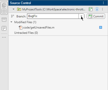
Source Control panel with a drop-down list next to the Branch field

Git API: Create local branch that tracks remote branch and switch to it in one step

When you attempt to switch to a branch that exists only in a remote repository, the switchBranch function can now automatically create a local branch and set the upstream branch to the remote tracking branch before switching to the new local branch.

repo = gitrepo;
branchDetails = switchBranch(repo,"remoteBranchName");
If the remote branch exists in more than one remote, specify which remote branch to track using the StartPoint name-value argument.
switchBranch(repo,"remoteBranch",StartPoint="origin/remoteBranch");

Git API: Specify SSH passphrase when you interact with Git repository

If your SSH key is passphrase protected, you can now specify the SSH passphrase when you programmatically interact with a Git repository using the gitclone, fetch, pull, and push functions. For example:

sshUrl = "git@github.com:user/examplerepo.git.";
gitclone(sshUrl,SSHUsername="user",SSHKeyPassphrase=getSecret("SSH_PASS"));

Git API: Clone single branch from Git repository

You can clone a single branch from a Git repository by specifying the new Branch and SingleBranch name-value arguments with the gitclone function.

url = "https://github.com/domain/examplerepo";
gitclone(url,Branch="FeatureB",SingleBranch=true);

Source Control: Sign Git commits using SSH keys

Starting in R2026a, MATLAB supports signing Git commits using SSH keys. For more information, see Configure Git Settings.

mpmuninstall Function: Delete uninstalled packages from disk

When you uninstall packages and their dependencies using the mpmuninstall function, you can specify the new Delete name-value argument as true to delete the corresponding package files and folders from disk.

Packages that are installed in-place are uninstalled but not deleted and must be removed from disk manually.

PackageIdentifier Object: Store package identifying information

Use the matlab.mpm.PackageIdentifier object to store the identity information of a specific package, including its name, version, and UUID. You can pass this object as an input to any MATLAB Package Manager function that accepts a package specifier.

Build Automation: Run tasks in parallel

When you run a build in parallel, either programmatically using the buildtool command or interactively from the MATLAB Toolstrip, the build tool executes tasks on the MATLAB client and workers in the current parallel pool (requires Parallel Computing Toolbox). Previously, running a build in parallel affected only how matlab.buildtool.tasks.TestTask instances ran.

The build tool considers task dependencies when scheduling a task to run in parallel. A task starts running in the parallel pool only after its dependencies have finished. For an example, see Run Tasks in Parallel.

Build Automation: View build summary in build output

When you run a build, the build output concludes with a build summary. The summary includes the outcome and duration of the build, as well as an overview of task execution. You can run a build either programmatically using the buildtool command or the run method of the matlab.buildtool.Plan class, or interactively from the MATLAB Toolstrip.

Build Automation: Control amount of build output interactively from Editor or MATLAB project

If your build file named buildfile.m is open in the MATLAB Editor or if your MATLAB project contains a build file named buildfile.m in its root folder, then you can interactively control the amount of information displayed during a build run from the MATLAB Toolstrip. For more information, see Run Build from Toolstrip.

Build Automation: Display test results in Test Browser

You can display the test results associated with matlab.buildtool.tasks.TestTask instances in the Test Browser app. To use the test browser when running a build, first select the Use Test Browser option in the Run Build section on the MATLAB Toolstrip. Then, run your TestTask instances interactively from the toolstrip or programmatically by specifying the -ui option of the buildtool command. For more information about the Use Test Browser option, see Run Build from Toolstrip.

Build Automation: Specify threshold for informational messages when identifying code issues

When identifying code issues using a matlab.buildtool.tasks.CodeIssuesTask instance, you can specify the maximum number of informational messages allowed for the task to pass by setting its InfoThreshold property. If the number of informational messages exceeds the specified threshold, then the task fails. You can set this property to perform stricter checks on your code. By default, a CodeIssuesTask instance does not fail on informational messages.

Unit Testing Framework: Add tests from currently open project to Test Browser

You can add the tests from the currently open MATLAB project to the Test Browser app. To automatically add the tests defined in project files and folders with the Test label, click the drop-down arrow to the right of the Add tests button on the Test Browser toolbar and then select Current Project. To also include the tests from referenced projects, select Include Referenced Projects.

Unit Testing Framework: Add tests to Test Browser by dragging files and folders

You can add tests to the Test Browser app by dragging test files and folders from the Files or Project panel into the Test Browser panel. To include the tests in the subfolders of a dragged folder, first click the drop-down arrow to the right of the Add tests button on the Test Browser toolbar and select Include Subfolders.

Unit Testing Framework: Automatically open MATLAB project when running tests in project files and folders

If you run tests from test files and folders that belong to a MATLAB project, and that project is not already open, then the testing framework automatically opens the project before running the tests and closes the project afterward. This behavior occurs because the framework automatically includes a matlab.unittest.fixtures.ProjectFixture instance when creating a test suite from test files and folders in a MATLAB project.

Unit Testing Framework: Test using parameterization properties that contain no data values

Parameterization properties can now contain an empty cell array or a scalar structure with no fields. When creating a test suite, the testing framework automatically excludes all the tests associated with parameterization properties that contain no data values. For an example, see Use External Parameters in Parameterized Test.

Unit Testing Framework: Generate test reports that have an improved appearance

Test reports generated using methods of the matlab.unittest.plugins.TestReportPlugin or matlab.unittest.TestResult class have an improved appearance. The improvements include a redesigned cover page and support for viewing the contents in light or dark theme.

The testing framework automatically selects colors that are visually appropriate for the theme. For example, text appears dark in light theme and light in dark theme. The theme of a report depends on where you view it:

  • A PDF or DOCX test report uses the theme of the application that renders it.

  • An HTML test report uses the theme of the MATLAB desktop. You can use the Toggle Theme switch at the top-left corner of the report to toggle between light and dark themes.

App Testing Framework: Programmatically interact with system dialog boxes

You can now use the chooseDialog and dismissDialog methods to programmatically interact with system dialog boxes created with the uigetdir, uigetfile, and uiputfile functions.

For example, create a test case for interactive testing.

testCase = matlab.uitest.TestCase.forInteractiveUse;

Dismiss the file selection dialog box that opens to the current folder.

dialogData = dismissDialog(testCase,"uigetfile",@uigetfile);

Select the bin folder in the folder selection dialog box that opens to the MATLAB root folder.

dialogData = chooseDialog(testCase,"uigetdir", ...
    @() uigetdir(matlabroot,"MATLAB Root Folder"), ...
    Folder=fullfile(matlabroot,"bin"));

App Testing Framework: Test Shift+click to select range of list box items

You can programmatically select a range of contiguous items in a list box by using the choose method. The choose method simulates the Shift+click action to select contiguous list box items. For an example, see Select Multiple Items in List Box.

App Testing Framework: Interact with table row and column headers

You can now programmatically interact with table row and column headers by using the press method. The method allows you to click a table row or column header to select the corresponding row or column, or click a sortable column header to sort the data in that column. For an example, see Press Table Headers.

Mocking Framework: Create mocks for classes with abstract WeakHandle properties

You can create mocks for classes that have properties with both the Abstract and WeakHandle attributes. For an example, see Create Mock for Class with Abstract WeakHandle Property.

 Functionality being removed or changed

mpmuninstall function returns an error for a package that is a dependency

Behavior change

If you attempt to uninstall an installed package that is a dependency of another package, the mpmuninstall function now returns an error.

Previously, if a package that was installed as a standalone package was also a dependency of another installed package, then calling mpmuninstall on that package did not uninstall the package but did change the InstalledAsDependency property to true.

matlab.addons.toolbox.toolboxVersion function no longer supports toolbox project files

Behavior change

When querying or modifying a toolbox version with the matlab.addons.toolbox.toolboxVersion function, you can now specify the toolbox file as a MATLAB project file that contains a toolbox task. As part of this change, toolbox project files (.prj) are no longer supported. To upgrade toolbox project files to MATLAB project files with a toolbox task, open the toolbox project file as a project in MATLAB. For more information, see Create and Share Toolboxes.

External Language Interfaces

 External Languages Panel: View, create, and manage Python environments in MATLAB

You can use the new External Languages panel to manage external programming language environments in MATLAB. Starting in R2026a, you can add Python environments, create virtual environments, switch between environments and execution modes, and manage libraries within Python environments.

To open the External Languages panel, click the Open more panels button on any sidebar and select External Languages. To manage Python environments using the External Languages panel, select the Python option from the menu at the upper left. For more information, see Manage Python Environments Using External Languages Panel.
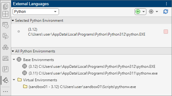
External Languages panel showing the selected Python environment as well as a list of all Python environments. The panel includes options to select an external language, add environments, manage settings, and refresh the panel view.

Call .NET from MATLAB: Unload .NET Core assembly from MATLAB

To unload a .NET Core assembly, set the Unloadable parameter to true when you call NET.addAssembly and then call NET.unloadAssembly.

You cannot unload a .NET Framework assembly.

Call .NET from MATLAB: Compare two .NET objects for equality

isequal and isequaln can now compare two .NET objects. You can use these functions to determine the equality of:

  • Two .NET objects

  • A .NET object and a MATLAB object that can be converted to a .NET object

In previous releases, isequal and isequaln do not support the comparison of .NET objects.

Python: Support for CPython version 3.13

MATLAB now supports CPython version 3.13, in addition to existing support for versions 3.9, 3.10, 3.11, and 3.12. For supported version information, see Versions of Python Compatible with MATLAB Products by Release.

Call Python from MATLAB: Automatically convert MATLAB string array to Python list

When you pass data to a Python function, MATLAB automatically converts 1-by-N or N-by-1 MATLAB string arrays to Python lists.

For example, MATLAB converts the string array mlArr to a Python list.

mlArr = ["apple", "banana", "cherry"];
pyArrType = py.type(mlArr);
For more information, see Pass Data Between MATLAB and Python from MATLAB.

pystringarray Function: Convert MATLAB string arrays to NumPy string arrays

You can create a NumPy StringDType array from a multidimensional MATLAB string array by using the pystringarray function. The pystringarray function requires NumPy 2.0 or greater.

Call Python from MATLAB: Compare two Python objects for equality

As of MATLAB R2024b, isequal and isequaln can compare two Python objects. You can use these functions to determine the equality of:

  • Two Python objects

  • A Python object and a MATLAB object that can be converted to a Python object

  • Two NumPy arrays

  • A NumPy array and a MATLAB array

In previous releases, isequal and isequaln do not support the comparison of Python objects.

 Call Java from MATLAB: Configure JRE for the MATLAB Support for OpenJDK add-on

The -clear option in the jenv and matlab_jenv functions removes the current JRE configuration for individual users or for each MATLAB installation for all users. After you install the MATLAB Support for OpenJDK add-on from the Add-On Explorer, use the -clear option so that MATLAB uses the add-on. For more information, see Configure Your System to Use Java.

 Compatibility Considerations

If you call jenv or matlab_jenv with the Java version argument set to "factory", MATLAB sets the Java path to the version included with MATLAB. However, in a future release, MATLAB will no longer include Oracle Java as part of its installation, and the argument value "factory" will be removed. Likewise, the JavaEnvironment Configuration property value "factory" will be removed.

Call MATLAB from C++: Run MATLAB and your C++ application in the same process

You can run MATLAB in the same process as your C++ application. Call either matlab::engine::startMATLAB or matlab::engine::startMATLABAsync with mode set to MATLABApplicationMode::IN_PROCESS. To run MATLAB in-process on Mac, you must also use matlab::engine::runMacLoopInProcess to start MATLAB on the main thread of the process and run your application logic on a secondary thread.

Call MATLAB from C++: Support for matlab::data::Array data types in matlab::engine::MATLABEngine functions feval and fevalAsync

The matlab::engine::MATLABEngine member functions feval and fevalAsync support these matlab::data::Array data types:

For more information, see the RhsArgs&&... rhsArgs entry in the feval and fevalAsync Parameters tables.

Web Services: Specify how to handle a basic authentication header

You can choose how a RESTful function treats a basic authentication header. By default, a RESTful function first makes a request without credentials, receives a response that indicates supported authentication methods, and then makes a second request using a supported method. To specify that the RESTful function instead make the first request with a Basic Authentication header field, create a weboptions object with the BasicAuthenticationMethod name-value argument specified as "preemptive". For more information, see weboptions.

MEX Functions: Build MEX functions from free-form Fortran source code

The mex command builds MEX functions from both fixed-form and free-form Fortran source code. Free-form Fortran files typically use the .F90 extension.

Compilers: Support for MinGW-w64 version 14.2 compiler on Windows, Microsoft Visual Studio 2026, and Intel oneAPI 2025 compiler

MATLAB supports the MinGW®-w64 version 14.2 compiler on Windows platforms. You can use this compiler to build C and C++ interfaces, MEX files, and standalone MATLAB engine and MAT-file applications. For installation instructions, see MATLAB Support for MinGW-w64 C/C++/Fortran Compiler.

MATLAB also supports Microsoft Visual Studio 2026.

As of R2025b, MATLAB supports these Intel compilers:

  • oneAPI 2025 compiler with Microsoft Visual Studio 2019 and 2022

  • oneAPI 2025 compiler for Fortran with Visual Studio 2019 and 2022

For continued support for building your applications, consider upgrading to a supported compiler. For an up-to-date list of supported compilers, see Supported and Compatible Compilers.

Perl 5.42.0: MATLAB support on Windows

As of R2025b, MATLAB for Windows includes an updated version of Perl, version 5.42.0.

If you use the perl command on Windows platforms, see https://www.perl.org/ for information about using this version of the Perl programming language.

 Functionality being removed or changed

mex command will build MEX functions with the interleaved complex API by default

Behavior change in future release

In a future release of MATLAB, the default api option for the mex command will change to the interleaved complex API (-R2018a). To prepare for the upcoming change, it is recommended that you create new MEX files and update existing MEX files to use the interleaved complex API. For more information, see MATLAB Support for Interleaved Complex API in MEX Functions.

If you want to continue using the separate complex API (-R2017b), then explicitly specify the -R2017b option in your mex command. For example, build MEX file myMexFile.c using the standard complex API.

mex -R2017b myMexFile.c

For more information, see Upgrade MEX Files to Use Interleaved Complex API.

matlab.wsdl.createWSDLClient and matlab.wsdl.setWSDLToolPath will be removed

Still runs

The matlab.wsdl.createWSDLClient and matlab.wsdl.setWSDLToolPath functions will be removed in a future release.

Use the MATLAB RESTful functions (webread and webwrite) or the MATLAB HTTP interface instead. For more information, see Call Web Services from MATLAB Using HTTP.

Hardware Support

Arduino Hardware: Support for Arduino Nano ESP32 and ESP32-S3-DevKitM-1 boards

You can now use MATLAB Support Package for Arduino Hardware to communicate with the Arduino Nano ESP32 and ESP32-S3-DevKitM-1 boards over USB, Bluetooth, and Wi-Fi from an installed version of MATLAB. For more information on how to configure ESP32 boards, see Set Up and Configure ESP32 Hardware.

However, you cannot use the support package to connect these boards with an Adafruit Motor Shield V2, motor carrier, CAN interface, or serial devices. The function playTone and the name-value argument AnalogReferenceMode of the arduino object in external mode do not support these boards. For more information, see Supported Boards.

Arduino Hardware: Support for Raspberry Pi Pico and Pico W boards

You can now use MATLAB Support Package for Arduino Hardware to communicate with the Raspberry Pi Pico boards over USB and the Pico W boards over USB and Wi-Fi in the MATLAB desktop environment. For more information, see Supported Boards.

Arduino Hardware: Support for Wi-Fi in MATLAB Online

You can now use MATLAB Support Package for Arduino Hardware to communicate with supported Arduino boards over Wi-Fi in MATLAB Online. For more information on the boards that support Wi-Fi, see Supported Arduino Boards, Workflows, and Platforms on MATLAB Online.

Arduino Hardware: Bluetooth support for Arduino Uno R4 Wi-Fi board

You can now use MATLAB Support Package for Arduino Hardware to communicate with the Arduino Uno R4 Wi-Fi board over Bluetooth. For more information, see Supported Boards.

Arduino Hardware: New example to estimate battery state of charge using deep learning

This release includes a new example that uses MATLAB Support Package for Arduino Hardware with Deep Learning Toolbox™. For more information, see Estimate Battery State of Charge Using Deep Learning with ESP32 Board.

R2025b

New Features, Bug Fixes

Quality and stability improvements

R2025b delivers quality and stability improvements, building on the new features introduced in R2025a.

getframe Function: Improved performance when capturing frames in loop

Capturing frames in a loop using the getframe function shows improved performance. The improvement becomes more noticeable as the size of the figure and number of frames increase.

For example, create a figure that is 1074-by-647 pixels in size and plot a surface. Change the shape of the surface 100 times in a loop, and capture a frame in each iteration. This code is about 1.5x faster than in the previous release.

function timingCaptureFrames
f = figure(Position=[0 0 1074 647]);
Z = peaks;
s = surf(Z);
loops = 100;
M(loops) = struct(cdata=[],colormap=[]);
axis tight manual
tic
for k = 1:loops
    Zframe = sin(k*pi/10)*Z;
    s.ZData = Zframe;
    M(k) = getframe(f);
end
toc
end

The approximate execution times are:

R2025a: 7.79 s

R2025b: 5.18 s

The code was timed on a Windows 11, Intel Core i7-8665U CPU 8-Core Processor @ 1.90 GHz test system with a Microsoft Remote Display Adapter and Intel UHD Graphics 620 by calling the timingCaptureFrames function.

MATLAB Support Package for Quantum Computing: Solve knapsack and traveling salesperson problems using QUBO (September 2025, Version 25.2.0)

You can solve knapsack and traveling salesperson problems as QUBO problems. Convert the knapsack or traveling salesperson problem to an equivalent QUBO formulation using the knapsack2qubo or tsp2qubo function, respectively, which returns a qubo object. Solve the QUBO problem by using the solve function, which returns a quboResult object. You can then convert the QUBO result back to the knapsack or traveling salesperson formulation using the quboResult2knapsack or quboResult2tsp function, respectively.

MATLAB Support Package for Quantum Computing: Calculate expectation values using quantum devices (November 2025, Version 25.2.1)

When you run a quantum circuit using the run function, you can specify the possible Pauli basis measurement results by using the new Observable name-value argument. If you specify Observable, then the run function returns a QuantumTaskAWS or QuantumTaskIBM object whose result is the expectation value of measuring the quantum circuit in the basis specified by the observable. You can then retrieve the result of the quantum task object as a numeric expectation value using the fetchOutput function.

R2025a

New Features, Bug Fixes, Compatibility Considerations

Environment

 MATLAB Desktop: Access desktop using new layout with customizable sidebars

In R2025a, the MATLAB desktop has a new layout designed to improve productivity and streamline workflows. The new layout includes customizable sidebars on the left, right, and bottom of the desktop. The sidebars show the tools, such as the Files panel (previously referred to as the Current Folder browser), the Workspace panel, and the Command Window, that are docked in the desktop.

You can use the sidebars to access the desktop tools in panels and change the desktop layout. For example, to show or hide a panel, click its icon on the sidebar. To move a panel, drag the panel's title bar or sidebar icon to the left, right, or bottom of the desktop. To open a panel that is not already open, click the Open more panels button in any sidebar. Then, in the Open Panel dialog box, select from the available panels.

For more information about how to configure your desktop, see Configure the Desktop.
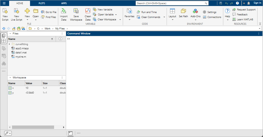
MATLAB desktop in R2025a. The left sidebar shows five panel icons, two of which are grouped together and enabled. The bottom sidebar shows one panel icon for the Command Window. The Command Window is open above the bottom sidebar. The Files panel and the Workspace panel are open on the left side of the desktop.

As part of this change, undocking some tools, such as the Files panel and Workspace panel, is no longer supported. Undocking the Command Window, Find Files panel, and Variables editor is still supported. In addition, customized layouts saved in a previous release of MATLAB are not supported.

 Desktop Themes: Change MATLAB desktop colors by selecting dark or light theme

You can change the colors of the MATLAB desktop using themes. For example, to select the dark theme, on the Home tab, in the Environment section, click Settings. Select MATLAB > Appearance and set Desktop Theme to Dark.

For more information, see Change Desktop Theme and Colors.
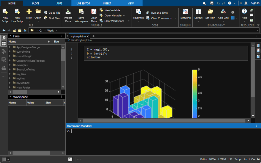
MATLAB desktop with a dark background and light text

 Desktop Accessibility: Use screen reader and keyboard to interact with different desktop areas

You can use a screen reader and keyboard to interact with the Command Window, navigate through the MATLAB desktop tools, and create and edit files in the Editor and Live Editor.

For more information, see Accessibility in MATLAB.

 Desktop Search: Access toolstrip actions, settings, and Help Center resources using search

You can now use the search box in the top-right corner of the desktop to easily access toolstrip actions, settings, and Help Center resources such as functions, blocks, examples, answers, and videos. To navigate to the search box using a keyboard, press Ctrl+Shift+Space (or Command+Shift+Space on macOS systems).

For example, to restore the MATLAB desktop to its default layout, type the word layout in the search box. In the list of results, select the Layout - Two Column (Default) toolstrip action.

Search box containing the word layout and a list of search results including toolstrip actions, functions, blocks, and examples

 Live Editor File Format: Create live scripts using new plain text file format

You can now create and save live scripts and functions using a plain text file format (.m). This new file format for live scripts improves integration with source control and allows you to open live scripts in external text editors.

Live scripts saved using the plain text file format behave just like other live scripts. They open in the Live Editor and can contain code, output, and formatted text. They also can include interactive controls and tasks.

For more information, see Live Code File Format (.m).
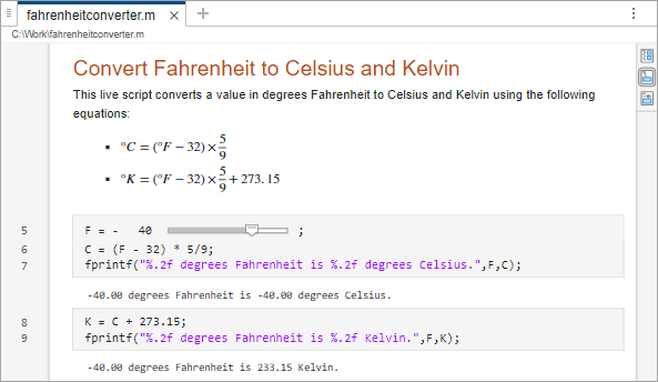
Live script with a .m file extension in the Live Editor. The live script contains formatted text, code, and output.

Live Editor Videos: Add YouTube videos and video files to your live scripts

You can add YouTube® videos and video files to your live scripts. Online videos are subject to the terms of service and privacy policy of the video provider.

To add a video to a live script, go to the Insert tab, and select Video > Online Video or Video > Video File. You can add videos only in text lines. If you insert a video in a code line, the Live Editor places it in a text line below the current code line.
Live script in the Live Editor containing text and a YouTube video with a play button

MATLAB Settings: Use Settings window to search for and modify MATLAB settings

MATLAB preferences are now renamed as settings, and you can search for and modify these settings using the updated Settings window. To open the Settings window, go to the Home tab, and in the Environment section, click Settings.

For more information, see Settings Window.
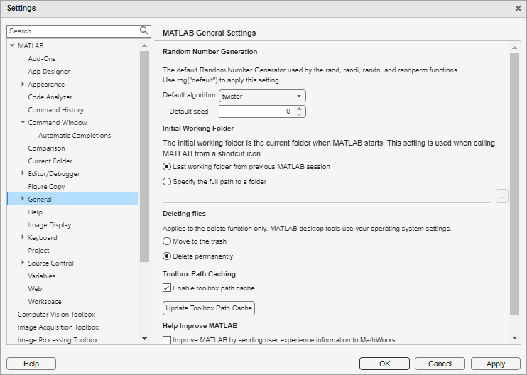
Settings window displaying the MATLAB General Settings page

Command Window: Show code suggestions automatically

Starting in R2025a, when you write code in the Command Window, MATLAB automatically provides real-time suggestions as you type. These suggestions include the names of functions, models, MATLAB objects, files, folders, variables, structures, and graphics properties. In addition, when you type a function name, MATLAB shows basic syntax information for the function and offers suggestions for parameters and options.

To disable or change the default behavior of code suggestions in the Command Window, go to the Home tab, and in the Environment section, click Settings. Select MATLAB > Command Window > Suggestions and in the Suggestions section, configure the settings based on your preferences.

For more information, see Code Suggestions.

Partially completed call to the plot function in the Command Window, with a list of suggested values for the LineStyle name-value argument

As part of this change, the Function browser and the Browse for functions button have been removed. To find functions, use code suggestions or the search box in the top-right corner of the MATLAB desktop.

Editor Markdown Support: Preview Markdown files in the Editor

When you open a Markdown file in MATLAB, the Editor shows a preview of the file to the right of the Markdown file. As you make edits to the file, the Editor updates the preview. To close the preview, go to the View tab and in the Preview section, click the Markdown button off.
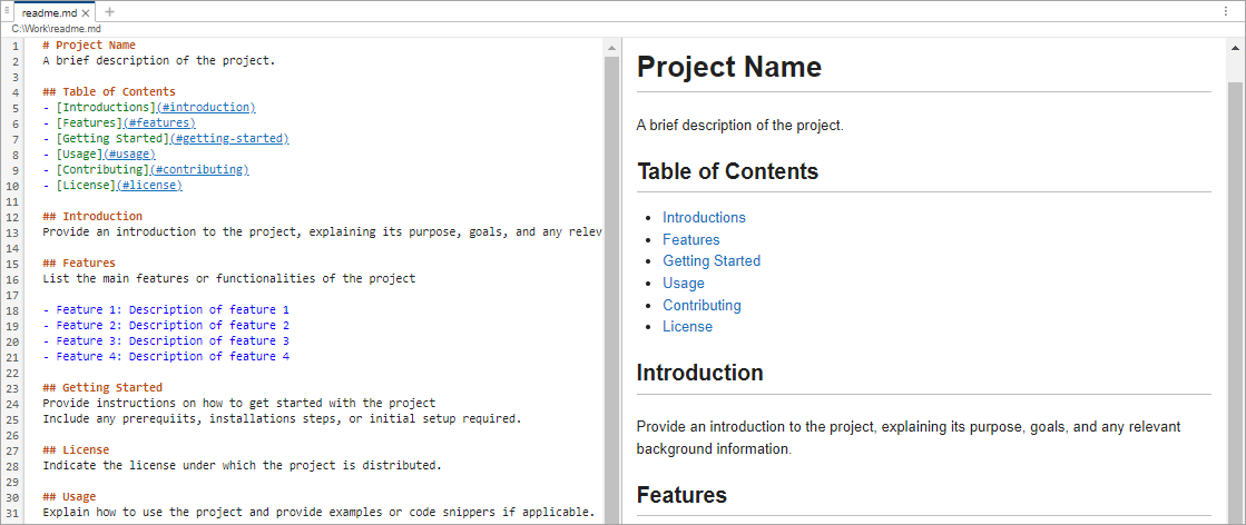
Markdown file readme.md with markdown for a title, section headers, and a bulleted list. To the right of the file is a preview of the file showing the formatted title, section headers, and bulleted list.

Editor Code: Insert code snippets

Code snippets are templates designed to simplify adding recurring code structures, such as loops or conditional statements, to your code. As you type in the Editor or Live Editor, MATLAB shows relevant code snippets along with other name suggestions. For example, if you type the word if, MATLAB suggests the If-Else Statement and If Statement snippets in addition to functions whose name starts with if.
File in the MATLAB Editor showing the typed characters "if" and a list of suggestions. The If-Else Statement snippet is selected in the list and a preview of the snippet code is visible next to the list of suggestions.

Editor Code: Copy code line without selection

You can copy a line of code in the Editor, Live Editor, and App Designer without selecting the code. To copy a code line, use the Ctrl+L keyboard shortcut. To cut a code line, use the Ctrl+X keyboard shortcut. On macOS, use the Command+C and Command+X keyboard shortcuts instead.

Outline Panel: View outline of your code using Outline panel

The Outline panel provides a high-level outline of scripts, live scripts, functions, and classes. To view an outline of a file open in the Editor or Live Editor, go to the View tab, and in the Tools section, click Outline. To navigate to an area within your code file, double-click the related entry in the Outline panel.
Outline panel showing the outline of the BankAccount class, which includes four properties and five methods

Code Issues Panel: Check code for errors and warnings using Code Issues panel

You can use the Code Issues panel to view error and warning messages about your code. The Code Issues panel displays potential coding problems that the MATLAB Code Analyzer finds as it automatically checks your code. Using the Code Issues panel, you can choose to view the errors and warnings for the current file or for all open files. You also can filter the list of messages by type (error, warning, or info) as well as by message text.

To open the Code Issues panel, go to the Editor or Live Editor tab, and in the Analyze section, click Code Issues. By default, the Code Issues panel opens on the right side of the desktop. To hide the Code Issues panel, click the Code Issues icon on the sidebar.

Code Issues panel showing 3 errors, 2 warnings, and 11 info messages found in the lengthofline.m file

Find Files Panel: Search for and replace text in filenames and file content using Find Files panel

You can use the Find Files panel to search for text in filenames and file content. To search, click the Find Files icon on the left sidebar. When searching, you can choose whether to match the case of your search text as well as whether to match the whole word. You also can select what folder to search in and filter results by file extension.

To replace text in filenames and file content, click the expand button to the left of the search box to open the replace options. Replacing text is supported in text files (.txt) and MATLAB plain text code files (.m).

To open the Find Files panel in a separate window, click the Find Files actions button at the top of the Find Files panel and select Undock Find Files.

For more information, see Find Files.
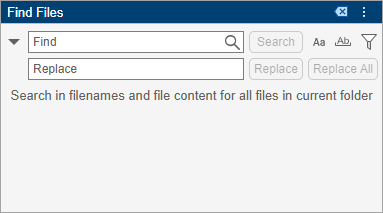
Find Files panel with a search box, a replace box, and options to match the case of the search text, match the whole word, and filter results

As part of this change, you can no longer exclude files from the search based on their file type or size.

Connections Panel: View and manage your connections using Connections panel

Use the Connections panel to view and manage your available connections, including OneDrive and MATLAB Drive. To open the Connections panel, click the Open more panels button on any sidebar and select the Connections panel.
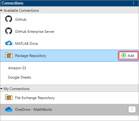
Connections panel with an Available Connections section and a My Connections section. The Available Connections section shows a Package Repository connection and an Add button to the right of the connection. The My Connections section of the panel shows MATLAB Drive and OneDrive connections.

Add-Ons Panel: Install and manage add-ons using Add-Ons panel

You can use the Add-Ons panel to find, install, and manage add-ons. You also can update an installed add-on, such as a support package, directly from the Add-Ons panel. To open the Add-Ons panel, click the Add-Ons icon on the left sidebar.

For more information, see Get and Manage Add-Ons.
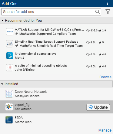
Add-Ons panel with a search box, a Recommended for You section with several recommended add-ons, and an Installed section with three installed add-ons. The second installed add-on has an Update button next to it.

Add-Ons Panel: View and install add-ons from MATLAB package repositories

You can view and install add-ons from MATLAB package repositories directly from the Add-Ons panel. To view and install the add-ons, click the Add-Ons actions button at the top of the Add-Ons panel and select Manage Package Repositories to open the Connections panel. In the Connections panel, add a connection to the MATLAB package repository. Then in the My Connections section, click the actions button to the right of the package repository connection and select Browse for Repository Add-Ons to return to the Add-Ons panel. In the Add-Ons panel, go to the From your Package Repositories section and select an add-on to install. You also can search for an add-on using the search box at the top of the panel.

For more information, see Install Add-Ons from MATLAB Package Repositories.
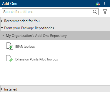
Add-Ons panel with a search box and a From your Package Repositories section showing three add-ons in a group named My Add-Ons

matlabProcessID Function: Get process identifier for MATLAB code execution process

Call the matlabProcessID function to get the process identifier for an active MATLAB process.

Window Managements in MATLAB Online: Use multiple browser tabs for MATLAB Online

In MATLAB Online, you can now open some files, apps, and tools in new browser tabs.

Using multiple browser tabs for MATLAB Online lets you:

  • Display MATLAB Online content on multiple monitors.

  • Seamlessly switch between multiple full-size MATLAB Online windows.

For more information, see Manage Windows in MATLAB Online.

Help Center: Get AI-generated response when searching the web documentation

When you search the web documentation, Help Center displays an AI-generated response along with the search results. The response includes:

  • A concise answer to your query

  • A list of sources used to generate the answer

  • A list of related searches for further exploration

AI-generated responses are based on relevant MathWorks documentation pages.

Folder Comparison: Compare folders and their subfolders recursively

When you select folders to compare, the Comparison Tool now includes the contents of all subfolders recursively in the comparison. To include only the folders you select and the first-level subfolders in the comparison report, in MATLAB, set the IncludeSubfolders comparison setting to false.

s = settings;
s.comparisons.folder.IncludeSubfolders.TemporaryValue = false;

For more information, see Compare Files and Folders and Merge Files.

matlab.crashhandling.crashReportFolder Function: Locate crash report folder

The new matlab.crashhandling.crashReportFolder function returns a path to the MATLAB crash report folder. Some crash files might be stored in other locations. For more information, see When MATLAB Terminates Unexpectedly.

 Functionality being removed or changed

matlab function -nojvm startup option supports desktop tools and graphics

Behavior change

If you start MATLAB using the matlab function with the -nojvm startup option, desktop tools and graphics appear as expected. In previous releases, desktop tools and graphics were not supported when MATLAB was started using the -nojvm startup option.

To prevent desktop tools and graphics from appearing, use the -nodisplay or -nodesktop options in addition to the -nojvm option. For example, this command starts MATLAB without the JVM software and without the desktop.

matlab -nojvm -nodisplay

matlab function no longer supports -nosplash startup option

Behavior change

The matlab function -nosplash startup option is no longer supported. If you specify the -nosplash option at startup, MATLAB ignores the option. Previously, you could use the -nosplash startup option to suppress the display of the splash screen.

Use monospaced font when running MATLAB using -nodesktop startup option

Behavior change

To ensure that output displays as intended when running MATLAB using the -nodesktop startup option on macOS or Linux, make sure that your macOS Terminal or Linux system prompt uses a monospaced font.

publish function no longer supports "entireFigureWindow" value for figureSnapMethod name-value argument

Errors

For the publish function, specifying the figureSnapMethod name-value argument as "entireFigureWindow" is no longer supported. Use the "entireGUIWindow", "print", or "getframe" values instead.

publish function no longer supports "bmp" value for imageFormat name-value argument with "pdf" format or "print" figureSnapMethod name-value argument

Errors

For the publish function, specifying the imageFormat name-value argument as "bmp" is no longer supported when the value of the format name-value argument is "pdf". With this change, you can instead specify imageFormat as either "png" or "jpg" for PDFs, with "png" being the default value. Specifying the imageFormat name-value argument as "bmp" is also no longer supported when the value of the figureSnapMethod name-value argument is "print".

Figures appear larger and as tabs by default in published documents

Behavior change

By default, figures created when publishing a document appear larger than in previous releases. In addition, these figures appear as tabs in a figure container.

To publish documents using the previous default figure size, set the Position property of each figure using a position vector of the form [left bottom width height]. Setting the Position property undocks the figure from the figure container.

f = figure(Position=[100 100 560 420]);

To use the previous default initial figure size for all figures, set the default figure position of the graphics root object.

set(groot,DefaultFigurePosition=[100 100 560 420])

For more information, see Figure.

Customizing quick access toolbar and Current Folder toolbar using Settings window is no longer supported

Behavior change

Customizing the quick access toolbar and Current Folder toolbar using the Settings window is no longer supported. In addition, moving the quick access toolbar is no longer supported. Previously, you could rearrange, add, and remove controls from both toolbars using the Settings window, and you could move the quick access toolbar below the MATLAB Toolstrip.

To rearrange controls in the quick access toolbar, drag them to the desired locations instead. To add a toolstrip control to the quick access toolbar, right-click the control and select Add to Quick Access Toolbar. You also can select from a list of common controls by going to the quick access toolbar and clicking the Common Controls button . To remove a control from the quick access toolbar, right-click the control and select Remove from Quick Access Toolbar.

There is no alternative way to customize the Current Folder toolbar.

Selecting and comparing files and folders from the Home tab has been removed

Behavior change

The Compare button on the Home tab that opens the Select Files or Folders for Comparison dialog box has been removed. To select files or folders on disk for comparison, use one of these methods instead:

  • MATLAB editors — Open a file in the MATLAB Editor or Live Editor. On the Editor or Live Editor tab, select Compare > Compare To. Then, select the file you want to compare to.

    You can also compare a file with the autosaved version or the saved version on disk. In the Editor tab, select Compare > Compare to Version on Disk or Compare to Backup. If you modified your file, the Editor saves the file before comparing. The Compare to Version on Disk and Compare to Backup options are available only if the option for automatically saving changes to a file is disabled. To disable the option, go to the Home tab, and in the Environment section, click Settings. Then, select Editor/Debugger > Saving and clear Save changes upon clicking away from a file. This option is not available in the Live Editor.

  • Files or Project panel — To compare two files on disk, select both files. Then, right-click and select Compare Selected Files/Folders. The Comparison Tool opens the file you select first on the left.

    Alternatively, right-click a file and select Compare To. Then, select the file you want to compare to.

  • Command Window — Use the visdiff function.

For more information, see Compare Files and Folders and Merge Files.

XML comparison report has been removed

Behavior change

When you compare two XML files, the Comparison Tool opens a text comparison report. For more information, see Compare Text Files.

Functions related to XML comparison, such as xmlcomp.compare, xmlcomp.zipTempFiles, and xmlcomp.showLogFile, will be removed in a future release. Starting in R2025a, these functions issue a warning.

XML comparison type for visdiff function has been removed

Errors

The XML comparison type for the visdiff function has been removed. Overriding the default comparison type by specifying "xml" is no longer supported. Starting in R2025a, the syntax visdiff(filename1,filename2,"xml") issues an error.

Command History saved to settings instead of history file

Behavior change

MATLAB now saves the Command History to settings. Previously, MATLAB saved the Command History to the history file History.xml in the settings folder. For more information, see Command History.

Language and Programming

 Debugging: Manage breakpoints and navigate function call stack using Debugger panel

Use the Debugger panel to manage breakpoints and navigate the function call stack while debugging. To open the Debugger panel, go to the Editor or Live Editor tab, and in the Analyze section, click Debugger. You also can open the panel using the Open more panels button on the sidebar.

For more information, see Debug MATLAB Code Files.
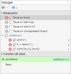
Debugger panel showing a Breakpoints section and a Function call stack section. The Breakpoints section shows Pause on Errors selected, as well as three enabled breakpoints in the plotRand.m file. The Function call stack section shows that the debugger is paused at line 3 of plotRand.m.

 MATLAB Identifiers: Maximum length of MATLAB identifiers increased to 2048 characters

The maximum allowed identifier length has increased to 2048 characters. This change allows variables, functions, classes, and many other entities to have names of up to 2048 characters. You can query the maximum identifier length by using the namelengthmax function.

Using longer identifiers might negatively impact performance and memory. Operating systems might have maximum filename lengths that are shorter than this limit.

 Compatibility Considerations

Previously, the maximum length of identifiers was 63 characters. Code that depends on identifiers being truncated to 63 characters might no longer run as expected.

cell2mat function accepts larger set of data types

Before R2025a, cell2mat accepted numeric, logical, and character types, as well as structures with the same field names. All cells of the input array had to have the same data type.

cell2mat can now accept cell arrays containing additional data types, including strings, categoricals, gpuArray objects, and class-based objects.

The function can also convert a cell array that contains different data types if MATLAB can convert those data types to one output type. For examples of basic data type combinations and their resulting types, see Valid Combinations of Unlike Classes.

If the cell array contains class-based objects of different classes, MATLAB attempts to concatenate them. For more information, see Concatenating Objects of Different Classes.

onCleanup Object: Cancel cleanup tasks

The cancel object function cancels any cleanup tasks specified by the onCleanup object and prevents them from being executed when the object is destroyed.

matlab.lang.Workspace Object: Store workspace variables

Store variables within a workspace as a matlab.lang.Workspace object. You can pass this object and access it from other workspaces in the same way as any other variable. To create a workspace object, use one of these functions:

  • matlab.lang.Workspace.baseWorkspace - store variables from the base workspace. The base workspace contains variables that you create at the command line. The base workspace includes any variables that scripts create, if you run the script from the command line or from the Editor.

  • matlab.lang.Workspace.currentWorkspace - store variables from the current workspace. For instance, call matlab.lang.Workspace.currentWorkspace inside a function to save variables in the function workspace.

  • matlab.lang.Workspace.globalWorkspace - store global variables.

After you create a workspace object, you can use these object functions:

  • variables - Access information about workspace variables stored in a workspace object.

  • variableNames - Return the names of variables stored in a workspace object.

  • evaluateAndCapture - Evaluate code in the workspace represented by a workspace object.

secretID Object: Keep sensitive information encrypted when setting object properties

You can avoid saving credentials and other sensitive information as plain text in properties of objects such as weboptions by using a secretID object. First, save sensitive information to your MATLAB vault as a secret using setSecret. Then when you set an object property, such as the Password property of a weboptions object, use a secretID object to keep your sensitive information encrypted.

For example, if you save your password as a secret named "myPass", use a secretID object to set a property to your associated secret.

opts = weboptions;
opts.Password = secretID("myPass");

 Functionality being removed or changed

Defining classes: Using function syntax to define classes will not be supported in a future release

Still runs

Support for defining classes using function syntax will be removed in a future release. With appropriate code changes, replace existing function-based classes with classes defined using the classdef keyword.

Defining classes: Using schema.m will not be supported in a future release

Warns

Support for classes defined using schema.m files will be removed in a future release. Replace existing schema-based classes with classes defined using the classdef keyword.

Change in precedence for functions and classes in @-folders with the same name

Warns

In a future release, the rule giving precedence to a class defined in a class folder (@-folder) over a function of the same name, regardless of position on the path, will be removed. MATLAB now issues warnings when these three conditions are met:

  • You have a class defined in a class folder and a function with the same name on your path.

  • The function appears earlier in the path order than the class.

  • You use the name of the function and class.

For more information, see Precedence of Classes in @-folders over Functions of the Same Name Will Be Removed in a Future Release.

Data Analysis

 Variables Editor: View and analyze variable contents using improved interface

The Variables editor has new tools for navigating and analyzing variable contents. For example, you can:

  • View edits to variables of all types as MATLAB code in the Command Window.

  • View sparklines and summary statistics for data in a table or timetable.

  • Create a logical variable from selected data indices.

  • Navigate variable contents using the Find and Go To buttons on the toolstrip.

  • Create a linked plot that is synchronized with workspace variables.

  • Edit categories of a categorical table variable.

The Variables editor display has enhanced readability for some variable types. For example, you can:

  • Review and analyze data in a table, timetable, structure array, or cell array using a simplified, borderless design and row striping.

  • Edit the contents of and view useful information for data in a scalar structure, object array, or cell array.

  • Interactively edit each page of data in a multidimensional array.

  • View the event labels for data in a timetable.

You can open the Variables editor by double-clicking a variable in the Workspace panel or using the openvar function.
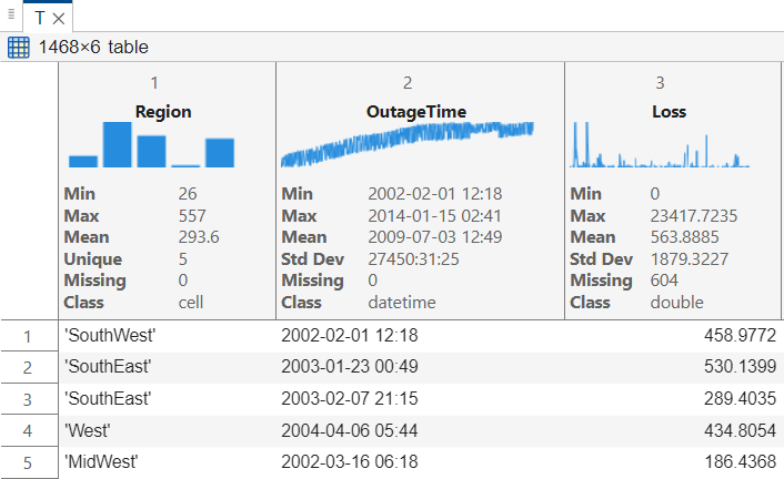
Variables editor view of a table with a borderless design and row striping. The header of each table variable displays a sparkline and summary statistics.

Figure Container: Organize, explore, customize, and generate code for plotted data using an improved figure window

Figures now open as tabs in a docked figure container in the MATLAB desktop by default. You can use the figure container to organize, explore, customize, and generate code for plotted data more efficiently:

  • Quickly customize and annotate figures using the toolstrip of the figure container.

  • Automatically generate code to reproduce figure interactions and customizations.

  • View figures more easily with their larger default size and wider aspect ratio.

  • Customize the layout of open figures by rearranging their tabs, or view multiple figures simultaneously by arranging them in tiles.

For more information, see Interactively Explore and Analyze Plotted Data.

For compatibility considerations, see Figure Container: Figures appear larger and as tabs by default.

allbetween and mustBeBetween Functions: Determine if or validate that all elements are within specified range

You can check that elements in input data are within a specified range by using these functions:

  • allbetween — Return logical 1 (true) if all elements are within the specified range and return logical 0 (false) otherwise.

  • mustBeBetween — Validate that all elements are within the specified range and throw an error if any element is outside of the range.

For both functions, you can specify whether the upper and lower bounds are inclusive or exclusive. Additionally, for an input table or timetable, you can specify which variables to operate on using the DataVariables name-value argument.

numunique and allunique Functions: Count and verify unique values

You can count the number of unique values in input data and verify the uniqueness of all values in input data by using these functions:

  • numunique — Return the number of unique values.

  • allunique — Return logical 1 (true) if all values are unique and return logical 0 (false) otherwise.

unique Function: Specify set order and occurrence arguments together

For the unique function, you can specify in the same function call both the order of values in the returned set and whether the first or last index of a repeated value is returned. For example, in the function call [C,ia,ic] = unique(A,"stable","last"):

  • C contains the unique elements, ordered as in the input data A.

  • ia contains the indices of the last occurrence of these elements in A.

  • ic is a mapping from elements in C to elements in A.

Previously, specifying both the set order and occurrence arguments was not supported.

 table and timetable Data Types: Maximum length of dimension and variable names increased to 2048 characters

In tables and timetables, the maximum allowed length of dimension and variable names has increased to 2048 characters. This length matches the updated maximum identifier length, which you can query by using the namelengthmax function.

Using longer dimension and variable names in tables and timetables might negatively impact performance and memory.

 Compatibility Considerations

Previously, the maximum length of dimension and variable names in tables and timetables was 63 characters. Code that depends on dimension and variable names being no longer than 63 characters might not run as expected.

If you save a table or timetable with long dimension or variable names to a MAT file, then you can load it into a MATLAB release before R2025a. However, the earlier MATLAB release truncates the long dimension and variable names in the table or timetable to 63 characters.

Moving Statistics Functions: Calculate moving statistics for data in tables and timetables

You can calculate moving statistics for numeric data in tables and timetables. By default, moving statistics functions calculate statistics for all variables in a table or timetable. However, you can specify the variables to use for these calculations. Also, you can append results as new variables in the output.

These functions support moving statistics for table and timetable data:

prctile and quantile Functions: Calculate percentiles and quantiles using inclusive and exclusive methods

You can calculate percentiles and quantiles using an inclusive or exclusive method with the prctile and quantile functions. Specify the method name as "inclusive" or "exclusive", respectively. The "inclusive" method includes the 0th and 100th percentiles (or 0th and 1st quantiles) within the bounds of the data; the "exclusive" method excludes them.

Additionally, the name of the default method has changed from "exact" to "midpoint". The prctile and quantile functions continue to support Method="exact" for backward compatibility.

These examples illustrate the differences between the default method and the two new methods.

x = 1:5;
P = prctile(x,25,Method="midpoint")
P = 1.7500
x = 1:5;
P = prctile(x,25,Method="inclusive")
P = 2
x = 1:5;
P = prctile(x,25,Method="exclusive")
P = 1.5000

pivot Function and Pivot Table Live Editor Task: Rearrange data without aggregation

You can rearrange data that does not require aggregation, including nonnumeric data, by specifying the Method name-value argument of the pivot function as "none". When using the Pivot Table Live Editor task, select the No aggregation computation method in the Values pane of the Select pivot variables section.

For an example, see Rearrange Data Without Aggregation.

 Functionality being removed or changed

Specify page orientation when printing variable contents by using MATLAB Print dialog box

Behavior change

To specify the page orientation when printing the contents of a variable, use the options in the MATLAB Print dialog box. Page numbers are no longer printed in the page header, and all rows print before wrapped columns.

Previously, the Page Setup dialog box controlled the page orientation.

Plot Catalog tool has been removed

Behavior change

The Plot Catalog tool has been removed. To interactively create and explore visualizations for your data, use the Plots tab of the MATLAB Toolstrip or the Create Plot task in the Live Editor.

For more information about visualizations, see Types of MATLAB Plots or toolbox-specific documentation.

Variables editor displays properties of timeseries objects

Behavior change

When you open a timeseries object in the Variables editor, the editor now displays the Property, Value, Size, and Class columns directly, rather than displaying a specialized editor for the timeseries data. You can still access and view all the properties of the timeseries object and edit some of its property values using this updated display.

Variables editor no longer supports opening a variable that does not exist

Errors

The Variables editor no longer supports opening a variable that does not exist. For example, if the variable a does not exist, then openvar a returns an error.

Data Import and Export

Reading Compressed Data: Read data from compressed and archived files

You can read data from compressed and archived files as a table, cell array, matrix, struct, timetable, dictionary, string array, or variable. Specify ZIP, GZ, and TAR files when using these functions:

File Permissions: View and adjust file permissions

You can view the permissions of files, folders, and symbolic links using the filePermissions function. The data type of the returned permissions information depends on the system where the file, folder, or symbolic link is located. You can then get or set individual permissions by using the getPermissions and setPermissions functions, respectively.

Datastores: Specify multiple remote files using wildcard characters

You can create a datastore from multiple remote files. Specify multiple remote files using wildcard characters anywhere in the file path when creating tabularTextDatastore, spreadsheetDatastore, imageDatastore, parquetDatastore, and fileDatastore objects.

FTP and SFTP: Specify folders in server hostname

When connecting to an FTP or SFTP server using the ftp or sftp function, you can specify folder paths in the server hostname. For example, connect to a sample FTP server.

ftpobj = ftp("ftp.example.com/myfolder");

xslt Function: Specify XSLT processing engine for transforming an XML file

When transforming an XML file using the xslt function, you can specify the XSLT processing engine as either the MATLAB API for XML Processing (MAXP) or Java API for XML Processing (JAXP). In the xslt(__,XMLEngine=xmlengine) syntax, specify xmlengine as "maxp" or "jaxp", respectively.

HDF5 Interface: Read and write cloud-optimized HDF5 files

You can create HDF5 files that are optimized for the cloud by specifying file-space handling strategies, file-space page sizes, and page buffer sizes. A cloud-optimized HDF5 file has an internal structure that is arranged for more efficient data access when the file is in cloud object stores. Use these functions in the low-level HDF5 interface:

You can retrieve the file-space handling strategy, file-space page size, page buffer size, and minimum percentage for metadata and raw data pages for an HDF5 file. Use these functions in the low-level HDF5 interface:

To support cloud-optimized HDF5 files, the H5P.set_chunk_cache function accepts new values for three of its input arguments:

  • Specify nslots as "H5D_CHUNK_CACHE_NSLOTS_DEFAULT" to use the number of elements specified in the file access property list to open the file instead of setting the property on the dataset.

  • Specify nbytes as "H5D_CHUNK_CACHE_NBYTES_DEFAULT" to use the number of bytes specified in the file access property list to open the file instead of setting the property on the dataset.

  • Specify w0 as "H5D_CHUNK_CACHE_W0_DEFAULT" to use the preemption policy value specified in the file access property list to open the file instead of setting the property on the dataset.

Import Tool: Import data with timestamps as timetable

You can import timestamped data from a file as a timetable using the Import Tool. If the tool detects timestamps in the first variable of the data to import, the tool uses the timetable data type by default.

Image Files: Read and display HEIF and HEIC image files

You can now read HEIF and HEIC image files using the imread function. You can also use imfinfo to get information about HEIF and HEIC image files and imshow to display the HEIF and HEIC images.

This functionality requires MATLAB Support for HEIF/HEIC Image Format, which is available only on MATLAB desktop environment.

To install the support package:

  • On the MATLAB Home tab, in the Environment section, select Add-Ons > Explore Add-Ons.

  • In the Add-On Explorer search bar, search for MATLAB Support for HEIF/HEIC Image Format, and then click the MATLAB Support for HEIF/HEIC Image Format add-on.

 Functionality being removed or changed

fopen function no longer supports fopen("all") syntax

Errors

The fopen function returns an error if you use the fopen("all") syntax. To get the file identifiers of all open files, use the openedFiles function instead.

web function opens local pages and files in HTML Viewer instead of MATLAB web browser

Behavior change

When you use the web function to open a local URL or file, the page now opens in the HTML Viewer. Previously, the page opened in the MATLAB web browser. As part of this change, the MATLAB web browser has been removed.

web function returns handle to most recent MATLAB web browser as matlab.htmlviewer.HTMLViewer class

Behavior change

The web function now returns a handle to the most recent MATLAB web browser as a matlab.htmlviewer.HTMLViewer object. In previous releases, the web function returns the handle as an instance of a Java class. With this change, some methods that were previously supported in the returned handle are no longer supported.

In most cases, you do not need to make any changes to your code. However, if your code uses methods that are not supported in the returned matlab.htmlviewer.HTMLViewer class, you must update your code.

Import Tool no longer supports dragging a file to import

Behavior change

You can no longer drag a file into the Import Tool to import its data. To import data from a file using the Import Tool, right-click the file in the Files panel and select Import Data.

Import Tool imports text as string array

Behavior change

The Import Tool imports all text as string arrays, except for in cell arrays. Previously, you could choose to import text as either a string array or a cell array of character vectors.

Mathematics

 Sparse Matrix: Create and use single-precision sparse matrices

Single-precision sparse matrices are now supported in all functions that support double-precision sparse matrices, including elementary math, linear algebra, and sparse matrix functions. You can create a single-precision sparse matrix using these functions:

By default, these functions create a double-precision sparse matrix. To create single-precision sparse data, specify the new typename argument as "single". For example, create a 50-by-100 single-precision sparse matrix with density 0.1 by calling sprand(50,100,0.1,"single").

You can also create single-precision sparse matrices by providing single-precision input data to sparse. For example, create a 4-by-4 single-precision sparse matrix by calling sparse(1:4,1:4,single([3 4 5 6])).

 Compatibility Considerations

If you save a single-precision sparse matrix to a MAT file, you can load it into an earlier release of MATLAB. However, how the data is loaded depends on the release of MATLAB:

  • MATLAB R2021b through R2024b — MATLAB warns that the data has an unsupported data type and loads it as a double-precision sparse matrix.

  • MATLAB R2021a and earlier — MATLAB loads the data as a single-precision sparse matrix, but you cannot use the matrix because its data type is unsupported. Attempting to use the matrix can result in undefined behavior.

ode Object: Solve delay differential equations

You can solve delay differential equations (DDEs) using an ode object by specifying the Solver property as "dde23", "ddesd", or "ddensd" and specifying the DelayDefinition property as an odeDelay object. If you specify only DelayDefinition and not Solver, the ode object automatically selects a solver.

ode Object: Solve complex-valued functions

You can solve ordinary differential equations (ODEs) with complex solution values using an ode object by specifying the SeparateComplexParts property as "on". Specify SeparateComplexParts as "on" when the ODE is complex and the selected solver fails or takes a long time to converge. This is especially helpful for solving implicit and stiff ODEs where the Jacobian is not specified.

Solve ODE Live Editor Task: Detect stiffness and specify minimum step size

In the Solve ODE task, you can enable stiffness detection for problems where the task automatically selects the solver. In the Specify solver options section, select Detect stiffness when Solver is Automatic.

You also can specify a minimum step size when the selected solver includes the MinStep option. In the Specify solver options section, enter a value in the Min step box. For a summary of the available options for each solver, see the SolverOptions property of the ode object.

pdepe Function: Specify output function and other odeset options

You can now specify all odeset options, including the output function, when using the pdepe function. However, pdepe overrides values for the Mass, MStateDependence, MvPattern, MassSingular, Jacobian, JPattern, and Vectorized options when defining the PDE to solve.

pagelsqminnorm Function: Apply Tikhonov regularization to page-wise least-squares solution

You can apply Tikhonov regularization to the page-wise least-squares solution of the pagelsqminnorm function by specifying the regularization factor alpha as a real number or a multidimensional array. Specify alpha to return a solution X that minimizes pagenorm(A.*X-B).^2 + alpha.^2.*pagenorm(X).^2 for each column of each page of X, given coefficient and input arrays A and B.

 Functionality being removed or changed

Two-input syntax of diff function calculates differences along only the first dimension whose size is greater than 1

Behavior change

The two-input syntax diff(X,n) of the diff function now operates along only the first dimension of X whose size is greater than 1 for all values of n. If n is larger than that dimension, diff returns an empty array. For example, this code now returns a 0-by-3 empty double matrix.

X = [1 1 1; 5 5 5];
Y = diff(X,3);

Previously, when n was larger than the first dimension of X whose size is greater than 1, diff(X,n) reduced the size of that dimension to 1 and then calculated differences along the next dimension whose size is greater than 1. In previous releases, this code returned 0.

Three- and four-input syntaxes of spdiags function return output with data type that is more consistent with inputs

Behavior change

The output of the three-input syntax and the four-input syntax of the spdiags function is more consistent with the inputs, as shown in this table.

SyntaxOutput Type in R2024b and EarlierOutput Type Starting in R2025a
S = spdiags(Bin,d,A)
  • sparse logical if either Bin or A is logical

  • sparse double otherwise

Same as A
S = spdiags(Bin,d,m,n)
  • sparse logical if Bin is logical

  • sparse double if Bin is not logical

Same as Bin

For example, this code now returns a 5-by-5 sparse single matrix.

S = spdiags(single([-1 1]),[-1 1],5,5);

In previous releases, this code returned a 5-by-5 sparse double matrix.

colon operator no longer supports nonscalar operands

Errors

colon now returns an error when creating vectors if one or more operands are not scalar. For example, expressions like [1 2 3]:2:10 now error. Previously, colon used the first element of any nonscalar operands to evaluate the expression.

To preserve the behavior of previous releases, update your code to specify the first element of any nonscalar operands in place of those nonscalar operands. For example, this code now returns an error because size(A) is nonscalar.

A = randn(3,4);
v = 1:size(A);
In previous releases, this code was equivalent to v = 1:3 because size(A) returned the vector [3 4] and colon used only the size of the first dimension of A to evaluate the expression. To achieve the same result, explicitly specify the size of the first dimension of A as the operand.
v = 1:size(A,1);

As another example, this code also returns an error because id is nonscalar.

id = find([1 2 3 1 2 3] == 3);
v = 1:id;
In previous releases, this code was equivalent to v = 1:3 because find returned the vector [3 6] and colon used only the first element of this returned vector to evaluate the expression. To achieve the same result, explicitly specify the first element of the vector as the operand.
v = 1:id(1);
Alternatively, you can directly specify that find return only the first index.
id = find([1 2 3 1 2 3] == 3,1,"first");
v = 1:id;

If you have a vector of sorted values, you can also use the min function to access the first element of the vector. For example, this code now returns an error because strfind returns a vector.

path = 'matlab/users/username/examples';
topDirname = path(1:strfind(path,'/')-1);
To achieve the same result as in previous releases, use the min function on the sorted vector returned by strfind.
topDirname = path(1:min(strfind(path,'/'))-1);

pow2 and log2 functions will no longer accept complex inputs when you specify two inputs or two outputs

Warns

The pow2 and log2 functions issue a warning if you specify complex inputs when using the two-input or two-output syntax. Support for complex inputs in these syntaxes will be removed in a future release. In previous releases, the two-input syntax of pow2 and the two-output syntax of log2 ignored the imaginary parts of complex inputs and processed only the real parts.

To preserve the behavior of previous releases, use the real function to extract the real parts of complex inputs, as shown in this table.

Not Recommended (Warns)Recommended
X = 2 + 1i;
E = 2i;
Y = pow2(X,E);
X = 2 + 1i;
E = 2i;
Y = pow2(real(X),real(E));
X = 2 - 1i;
[F,E] = log2(X);
X = 2 - 1i;
[F,E] = log2(real(X));

Graphics

 Themes: Create graphics using light or dark theme

You can view and create figures in light or dark theme. When you create plots, MATLAB automatically selects colors that are visually appealing for the theme. By default, figures use the theme of the MATLAB desktop, but you can choose a different graphics theme.

Two figures containing identical donut charts. One figure has a light theme (light background), and the other figure has a dark theme (dark background). The colors of the chart and slice labels are optimized for viewing in the respective themes.

You can manage the colors of a chart and the theme of a figure in these ways:

  • theme function or the Theme property of the figure – Set and get the theme of a figure.

  • MATLAB Settings window – Configure themes for all figures.

  • fliplightness function – Flip the lightness of color values.

  • getTheme method – Get the theme of the figure for a ChartContainer subclass.

For more information, see Graphics and App Themes.
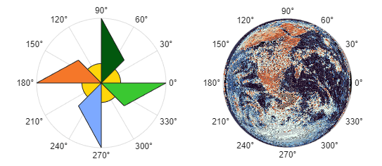
 Figure Container: Organize, explore, customize, and generate code for figures using an improved figure window

Figures now open as tabs docked in a figure container by default. You can use the figure container to organize, explore, customize, and generate code for figures more efficiently:

  • View figures more easily with their larger default size and wider aspect ratio.

  • Customize the layout of open figures by rearranging their tabs, or view multiple figures simultaneously by arranging them in tiles.

  • Quickly customize and annotate figures using the toolstrip of the figure container.

  • Automatically generate code to reproduce figure interactions and customizations.

For more information, see Interactively Customize Plot Appearance.

For compatibility considerations, see Figure Container: Figures appear larger and as tabs by default.

Polar Plots: Plot patches and surfaces in polar coordinates

Create patches and surfaces in polar coordinates by passing a PolarAxes object to the patch, pcolor, surf, surface, mesh, fill, and fill3 functions.

Two side-by-side polar plots. One polar plot contains four triangular patches in the shape of a pinwheel and a circle in the center. The second polar plot contains a surface with an image overlay of the earth.

Polar Plots: Specify location of zero degrees as an angle

Specify the location of zero degrees on the theta-axis as an angle value by setting the ThetaZeroLocation property of the PolarAxes object. You can assign a value such as 45 (when the ThetaAxisUnits property is "degrees") or pi/4 (when the ThetaAxisUnits property is "radians").

The ThetaZeroLocation property also supports its original options: "right", "left", "top", and "bottom".

colormaplist Function: List available colormaps

Return a list of predefined colormaps as a string array by using the colormaplist function.

nebula Function: Apply blue-to-red colormap to charts

Use the nebula function to get a blue-to-red colormap for coloring your charts. Like for all predefined colormaps, you can optionally specify the number of colors for the nebula colormap.
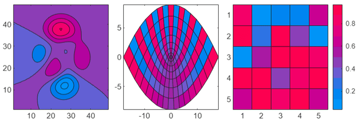
Three charts that use the nebula colormap

Pie Charts and Donut Charts: Choose text interpreter or no interpreter for titles and labels

Use LaTeX or TeX markup in the titles and labels of pie charts and donut charts by setting the Interpreter property of a PieChart or DonutChart object to "latex" or "tex". To display text without an interpreter, set this property to "none".

violinplot Function: Use additional grouping data options and customize color group appearance

You can now create violin plots from table and timetable data without specifying grouping variables. Use the new syntax violinplot(tbl,yvar) of the violinplot function to create violin plots from the yvar variables in table tbl.

You can also specify one shared set of sample data for multiple sets of positional grouping data. To share sample data coordinates, specify ydata as a vector and xgroupdata as a matrix in the syntax violinplot(xgroupdata,ydata).

In addition, you can customize the width and layout of color groups using these name-value arguments:

  • ColorGroupWidth — Adjust the space between each violin plot color grouping.

  • ColorGroupLayout — Specify whether to group or overlay the violin plots in each color grouping.

  • DensityWidth — Adjust the space between each overlaid color grouping.

boxchart Function: Create box charts using table data and customize box charts using additional properties

You can now create box charts from table and timetable data. Use the new syntax boxchart(tbl,yvar) of the boxchart function to create box charts from the yvar variables in table tbl. To create grouped box charts from a table, use boxchart(tbl,xvar,yvar), where the data in yvar is grouped by the data in xvar.

You can further customize the appearance of box chart whiskers as well as color groups using these name-value arguments:

  • CapWidth — Set the width of the whisker end caps.

  • ColorGroupWidth — Adjust the space between each box chart color grouping.

  • ColorGroupLayout — Specify whether to group or overlay the box charts in each color grouping.

  • BoxWidth — Adjust the space between each overlaid color grouping.

Swarm Charts: Create swarm charts with jitter in different directions

Set the XJitterDirection, YJitterDirection, and ZJitterDirection properties to control the direction of the jitter in a swarm chart. Each of these properties can have a value of "negative", "positive", or "both".
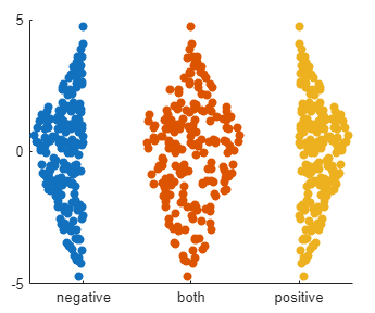
Three swarm charts plotted together. In the first chart, the points are jittered to the left (negative direction). In the second chart, the points are jittered to the left and right (both directions). In the third chart, the points are jittered to the right (positive direction).

Geographic Plots: Basemaps have improved appearance

The "streets-light", "streets-dark", "streets", and "topographic" basemaps hosted by Esri® have an improved appearance when the basemap tiles contain text. For example, this image compares a basemap in R2024b with the same basemap in R2025a. In R2025a, the labels for Wisconsin and St. Louis are fully visible.
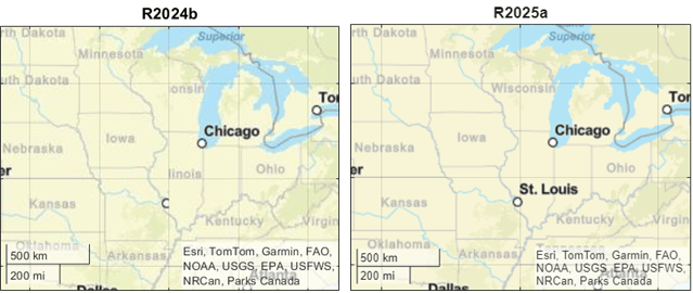
Comparison of basemaps in R2024b and R2025a

In addition, all cached basemap tiles have a crisper appearance. For more information about cached basemap tiles, see Access Basemaps for Geographic Axes and Charts.

tightPosition Function: Get location and size of axes plotting area in specific units

Get the location and size of the axes plotting area in specific units, such as pixel, inch, or centimeter units, by calling the tightPosition function with the Units name-value argument. For example, get the plotting area in inches.

ax = gca;
pos = tightPosition(ax,Units="inches");

exportgraphics and copygraphics Functions: Specify output dimensions using name-value arguments

Specify the width, height, padding, and whether to preserve the aspect ratio of the original graphic when you call the exportgraphics and copygraphics functions.

Use these name-value arguments to control these aspects of the content:

  • Width and Height — Specify the width and height of the output.

  • Padding — Specify the amount of padding around the perimeter of the graphic.

  • Units — Specify the units for the width, height, and padding values.

  • PreserveAspectRatio — Specify whether to automatically add padding to preserve the original aspect ratio if the Width and Height values conflict with the original aspect ratio of the graphic.

exportgraphics Function: Export plots as SVG files

Using the exportgraphics function, you can export a plot as an SVG file by specifying an ".svg" file extension in the filename. For example, export the contents of the current figure as an SVG file.

exportgraphics(gcf,"myfigure.svg")

getframe Function in MATLAB Online: Capture figures in MATLAB Online sessions

The getframe function is now supported in MATLAB Online. You can also use getframe to capture figures created with the uifigure function in any environment.

Copying Figures: Select options for copying figures in MATLAB Settings

Use the new Figure Copy page in the MATLAB Settings window to select options for copying figures to the clipboard. MATLAB uses these settings when you copy a figure using the figure toolstrip.

The new settings page includes these options:

  • Width and height in specified units

  • Image (pixels) or vector graphics

  • Resolution (for images)

  • Background color

  • Grayscale content

Titles and Labels: Use LaTeX to display math and symbols with more consistent results

As in previous releases, you can use the LaTeX interpreter to display text and labels in your graphics. Now, when you use markup in your graphics, the results are consistent across MATLAB. For more information, see Supported LaTeX Commands.

Text: Larger, easier-to-read text on macOS

Text in graphics has a larger, more readable default font size on macOS systems. The size is now consistent across Windows and macOS systems. Specifically, graphics objects that have a Units or FontUnits property set to "points", "inches", or "centimeters" display about 1.33x larger than their previous size on macOS systems.

For compatibility considerations, see Text: Text and other objects specified in "points", "inches", or "centimeters" are larger on macOS.

 Axes Interactions: Specify axes for interaction mode

In figures created using the figure function, you can set the interaction mode for axes. Specify the Axes object as the first argument for these functions:

For example, in a figure with two axes, enable pan mode for only the first axes.

f = figure;
t = tiledlayout(f,1,2);
ax1 = nexttile(t);
ax2 = nexttile(t);
pan(ax1,"on")

When setting the interaction mode for axes, these functions do not return pan, zoom, rotate3d, DataCursorManager, or brush objects. Previously, these functions set the interaction mode for all Axes children of the current or target figure.

 Compatibility Considerations

If you change an interaction mode for an Axes object in a figure, the interaction modes of other axes in that figure are not affected.

If you create a new plot in existing axes, interaction modes for the axes are now reset to their default values. Previously, creating a new plot in existing axes did not change the interaction mode for the figure.

Accessibility in MATLAB: Use screen reader to interact with figures

You can use a screen reader and keyboard commands to pan, zoom, and rotate when you work with plotted data. Using a screen reader to interact with figures is not supported in the Live Editor.

For more details on interacting with MATLAB figures, see Control Chart Interactivity.

 Graphics functionality being removed or changed

Figure Container: Figures appear larger and as tabs by default

Behavior change

By default, figures created using the figure function appear as tabs in a figure container. This change impacts the figures in these ways:

  • By default, the WindowStyle property of Figure objects is "docked" because the figures are docked in the figure container. In previous releases, the WindowStyle property was "normal" because figures were not docked by default.

  • By default, the figure container is undocked from the MATLAB desktop, and the figure container docked state does not persist between MATLAB sessions. In previous releases, the figure container was docked in the desktop by default, and the figure container docked state persisted between MATLAB sessions.

To create a figure window that is independent of other windows, specify the window style as "normal".

f = figure(WindowStyle="normal");

To dock the figure container into the desktop, click the Dock button in the top-right corner of the figure container.

In addition, figures have a larger default size that changes based on the size of your monitor. To use the previous default figure size for a single figure, set its Position property using a position vector of the form [left bottom width height]. Setting the Position property undocks the figure from the figure container.

f = figure(Position=[100 100 560 420]);

To use the previous default initial figure size for all figures, including those in the figure container, set the default figure position of the graphics root object.

set(groot,DefaultFigurePosition=[100 100 560 420])

Plot Appearance: Default colors for charts have changed slightly

Behavior change

Some of the default colors of graphics objects have changed. These changes affect the light theme colors. This table describes the changes and provides the RGB triplets and color samples to compare R2025a with the previous release.

Affected GraphicsAffected Object PropertiesR2024b ColorR2025a Color

Figure background color

Color property of Figure object

[0.94 0.94 0.94]

Sample of light gray color, the default figure background color (R2024b)

[0.9608 0.9608 0.9608]

Sample of slightly lighter gray color, the default figure background color (R2025a)

Plot colors

ColorOrder property of Axes object

(This property controls the default color of Line, Scatter, Bar, and other plot objects.)

RGB TripletSample

[0.0000 0.4470 0.7410]

Sample of dark blue color (R2024b)

[0.8500 0.3250 0.0980]

Sample of dark orange color (R2024b)

[0.9290 0.6940 0.1250]

Sample of dark yellow color (R2024b)

[0.4940 0.1840 0.5560]

Sample of dark purple color (R2024b)

[0.4660 0.6740 0.1880]

Sample of medium green color (R2024b)

[0.3010 0.7450 0.9330]

Sample of light blue color (R2024b)

[0.6350 0.0780 0.1840]

Sample of dark red color (R2024b)

RGB TripletSample

[0.0660 0.4430 0.7450]

Sample of dark blue color (R2025a)

[0.8660 0.3290 0.0000]

Sample of dark orange color (R2025a)

[0.9290 0.6940 0.1250]

Sample of dark yellow color (R2025a)

[0.5210 0.0860 0.8190]

Sample of dark purple color (R2025a)

[0.2310 0.6660 0.1960]

Sample of medium green color (R2025a)

[0.1840 0.7450 0.9370]

Sample of light blue color (R2025a)

[0.8190 0.0150 0.5450]

Sample of dark magenta color (R2025a)

Plot titles and annotations

Color property of Text or annotation object

[0 0 0]

Example of a plot title (R2024b)

[0.1294 0.1294 0.1294]

Example of a plot title (R2025a)

Axes labels, tick labels, and rulers

Axes labels: Color property of Text object

Axes tick labels and rulers: XColor, YColor, and ZColor properties of Axes object

[0.15 0.15 0.15]

Example of an x-axis with tick labels and a text label, "Distance", that describes the x-axis (R2024b)

[0.1294 0.1294 0.1294]

Example of an x-axis with tick labels and a text label, "Distance", that describes the x-axis (R2025a)

Rendering: opengl function, Renderer property, and renderer startup options have no effect

Behavior change

The following options for querying or setting the graphics renderer have no effect. MATLAB no longer uses OpenGL technology to render graphics, and you no longer need to set the renderer in your graphics workflows.

  • Calling the opengl function has no effect. To query the graphics renderer, use the rendererinfo function instead.

  • The Renderer property of a figure has no effect.

  • The MATLAB startup options -softwareopengl, -nosoftwareopengl, -softwareopenglmesa, and -noopengl have no effect.

The opengl function, Renderer property, and startup options will be removed in a future release.

Rendering: GraphicsSmoothing and FontSmoothing properties have no effect

Behavior change

The GraphicsSmoothing and FontSmoothing properties have no effect. All graphics and text are smooth regardless of the value of these properties.

  • The GraphicsSmoothing property of figures has no effect.

  • The FontSmoothing property of axes, rulers, geographic scales, and text objects has no effect.

These properties will be removed in a future release.

TeX and LaTeX Equations: Fonts and text spacing of equations have changed

Behavior change

The fonts and text spacing of some TeX and LaTeX equations and symbols have changed. For example, here are two paragraphs containing LaTeX equations and a fraction. The left paragraph shows the appearance in R2024b, and the right paragraph shows the same text in R2025a.

Content exported from a figure as vector graphics (SVG, PDF, EPS, or EMF files) continue to use the R2024b format in R2025a.

R2024bR2025a

Sample of a paragraph containing LaTeX equations and a fraction in R2024b. The equations use a small font that is about the same size as the surrounding text. The fraction uses a smaller font.

Sample of a paragraph containing LaTeX equations and a fraction in R2025a. The equations and the fraction use a larger font than the surrounding text, and there is more space above and below the lines containing math.

Text: Text and other objects specified in "points", "inches", or "centimeters" are larger on macOS

Behavior change

Graphics objects that have a Units or FontUnits property set to"points", "inches", or "centimeters" now use a conversion value of 1 pixel = 1/96 inch on macOS systems. Previously, the conversion value was 1 pixel = 1/72 inch. As a result, these objects have increased in size by a factor of 96/72 (about 1.33x). The new size provides consistency between macOS and Windows systems.

If you have code that uses the default ("normalized") units for positioning objects such as axes and annotations, those objects are unaffected by this change. However, text objects, such as titles and labels, appear larger by default on macOS systems. To preserve the sizes of text and other affected objects so that they match the sizes on macOS systems in previous releases, make these changes in your code:

  • Objects with Units or FontUnits set to "points" — Update the value of the property from "points" to "pixels".

  • Objects with Units or FontUnits set to "inches" — Update the value of the property from "inches" to "pixels" and multiply all Position values by 72.

  • Objects with Units or FontUnits set to "centimeters" — Update the value of the property from "centimeters" to "pixels" and multiply all Position values by 72/2.54.

Box Charts: Box widths are calculated based on input data

Behavior change

If you call the boxchart function without specifying the box width, MATLAB calculates the box width according to your data. In previous releases, the default box width was 0.5. To preserve the appearance from previous releases, specify the BoxWidth name-value argument as 0.5 when calling the boxchart function.

Color Utility Functions: The colordef, graymon, and whitebg functions have been removed

Errors

The colordef, graymon, and whitebg functions have been removed. To control the appearance of graphics in a figure, select a graphics theme. For more information, see Graphics and App Themes.

Modifying Plots: Plot tools are no longer supported

Errors

The Figure Palette, Plot Browser, and Property Editor tools have been removed or incorporated into the toolstrip of the figure container. As a result, these functions now return an error:

  • figurepalette

  • plotbrowser

  • propertyeditor

  • propedit

  • plottools

In addition, the "showtoolsmenu" and "hidetoolsmenu" options for the plotedit function return an error.

Instead, to interactively select graphics objects and modify their properties, you can enable plot edit mode and use the Property Inspector. To create a grid of axes in a figure, use the tiledlayout function. To create new charts within existing axes, use the Plots tab in the MATLAB Toolstrip and select the Reuse Figure option.

Figure Menu Bar: Menu bar no longer contains some menu items

Behavior change

For figures that display the menu bar instead of the toolstrip (for example, from setting the MenuBar property of the Figure object), the menu bar no longer contains the items described in this table.

Menu

Removed Item

Recommendation

File

  • Import Data

  • Save Workspace

Use the Variable section on the Home tab of the MATLAB Toolstrip.

Edit

  • Find Files

  • Clear Figure

  • Clear Command Window

  • Clear Command History

  • Clear Workspace

Use the File, Variable, and Code sections on the Home tab of the MATLAB Toolstrip.

View

  • Figure Palette

  • Plot Browser

  • Property Editor

See Modifying Plots: Plot tools are no longer supported.

Tools

  • Zoom In

  • Zoom Out

  • Pan

  • Rotate 3D

  • Data Tips

  • Restore View

  • Options

  • Align Distribute Tool

Interact with axes by using built-in axes interactions, or enable interaction modes by using the axes toolbar. Customize an interaction by right-clicking the chart when an interaction mode is enabled or by using the InteractionOptions property of the axes.

Control the arrangement of multiple axes in a figure by creating a tiled chart layout using the tiledlayout function.

Axes Interactions: Plot-box outline rotation is no longer supported

Behavior change

The plot-box outline rotation style for the rotate3d object is no longer supported. The rotation style rotates the entire axes, regardless of the value of the RotateStyle property.

Axes Interactions: Azimuth and elevation angles are not displayed by default

Behavior change

When you interactively rotate axes, the axes no longer display the azimuth and elevation angles by default. If you want to display these angles, in the InteractionOptions property of the axes, specify the RotateIndicator property as "azimuthelevation".

For example, create a 3-D plot and set its axes to display the azimuth and elevation angles during interactive rotation.

ax = axes;
surf(ax,peaks)
ax.InteractionOptions.RotateIndicator = "azimuthelevation";

Axes Interaction Modes: Enable property of interaction objects might be inaccurate

Behavior change

The Enable property of zoom, pan, rotate3d, and brush interaction objects might have a value of off when the interaction is enabled. If you want to determine whether the interaction mode is enabled, check the icons in the axes toolbar. If an interaction mode is enabled, its corresponding icon appears blue in the toolbar.

 Printing and exporting functionality being removed or changed

Printing: The print function no longer executes SizeChangedFcn callbacks

Behavior change

If you write a SizeChangedFcn callback for a figure, the callback no longer executes when you call the print function.

Exporting: The hgsave function and "compact" option of savefig will be removed

Warns

The hgsave function issues a warning that it will be removed in a future release. To save a FIG file, use the savefig function instead.

If you use the savefig function with the "compact" argument, the function issues a warning that the option will be removed in a future release. savefig saves compact FIG files regardless of whether you specify the "compact" option. These compact files are not compatible with releases prior to R2014b.

Exporting: The getframe function no longer captures figure borders or decorations

Errors

The getframe function returns an error if you use the rect argument to capture a region that is not fully contained within the drawable area of the figure. The drawable area is the area inside the borders of the figure and does not include the figure toolstrip.

Exporting: exportgraphics and copygraphics do not support adjacent containers

Behavior change

If you pass a container (such as a figure or panel) to the exportgraphics or copygraphics function, and that container has child containers, the function returns an error in some cases:

  • If there are multiple child containers, and at least one of the child containers has axes objects or standalone visualization objects in it

  • If the parent container has children that are axes objects (or standalone visualization objects) and those children are next to containers at the same level in the graphics hierarchy

To capture the contents of a child container, pass that container to the exportgraphics or copygraphics function. To capture all of the content of a figure, use the exportapp function.

Printing and Exporting: Background color of output no longer depends on InvertHardCopy property

Behavior change

The InvertHardCopy property of a figure has no effect. If you call the print or saveas function to save a figure to a file or copy it to the clipboard, the default background color corresponds to the theme of the figure. The background is white if the figure has the light theme. The background is dark gray (almost black) if the figure has the dark theme. If you set the Color property of the figure before calling print or saveas, the output uses the color you specify regardless of the theme.

If you call the print function to print a hard copy, the background color is white (no ink) by default. If you set the Color property of the figure, the output uses that color.

Printing and Exporting: The hgexport and printopt functions have been removed

Errors

The hgexport function has been removed. To save the contents of a plot as an image or vector graphics file, use the exportgraphics function. To copy the contents of a plot to the clipboard, use the copygraphics function. To save the contents of an app as an image file, use the exportapp function.

The printopt function has been removed. To configure printer defaults, use the options provided by your operating system.

Printing and Exporting: The print and saveas functions no longer support UI components and certain file types

Errors

The print and saveas functions no longer support capturing UI components or containers such as panels and tabs. The functions also no longer support BMP, HDF, PBM, PCX, PGM, PPM, or full-page PostScript® (.ps) files.

To export a figure containing UI components or containers, use the exportapp function instead. For example, this code creates a simple app and exports the figure as a PDF file.

% Create figure with three UI components
f = uifigure;
button1 = uibutton(f,Position=[150 300 100 50]);
button2 = uibutton(f,Position=[300 300 100 50]);
slider1 = uislider(f,Position=[150 250 250 3]);

% Export the contents of the figure
exportapp(f,"myapp.pdf")

To export a graphic as a BMP, HDF, PBM, PCX, PGM, or PPM file, use the getframe and imwrite functions instead. For example, this code exports a figure as a BMP file.

plot([0 3 2 4 1]);
F = getframe(gcf);
imwrite(F.cdata,"myplot.bmp");

To export vector graphics files, use the exportgraphics function. Specify an .svg, .eps, .pdf, or .emf file extension and set the ContentType name-value argument to "vector". For example, this code exports a figure as a PDF file.

plot([0 3 2 4 1]);
exportgraphics(gcf,"myplot.pdf",ContentType="vector")

Printing and Exporting: Figures shrink to fit page size and Renderer property has no effect on output

Behavior change

The print and saveas functions no longer clip the contents of a large figure when the page is smaller than the figure. Now, these functions shrink the content to fit on the page and preserve the aspect ratio of the figure.

The Renderer property of a figure has no effect on the output produced by the print and saveas functions.

App Building

 Themes: Create apps and custom UI components using light or dark theme

You can view and create figures in light or dark theme. When you create UI components and plots, MATLAB automatically selects colors that are visually appealing for the theme. By default, figures use the theme of the MATLAB desktop, but you can choose a different graphics theme.
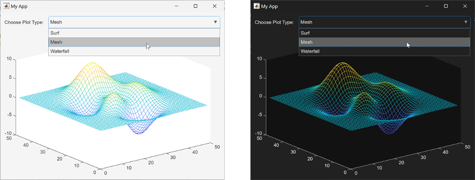
Two figures containing an identical drop-down component and chart. One figure has a light theme (light background), and the other figure has a dark theme (dark background). The colors of the component, chart, axes, and text are optimized for viewing in the respective themes.

You can manage the colors and themes of your apps in these ways:

  • theme function or Theme property of the figure — Set and get the theme of a figure.

  • MATLAB Settings window — Configure themes for all figures.

  • ThemeChangedFcn property of the figure — Program response to figure theme change.

  • fliplightness function — Flip the lightness of color values.

  • getTheme method — Get the theme of the figure for a ComponentContainer class.

For more information, see Graphics and App Themes.

uiprintdlg and uiexportdlg Functions: Open dialog boxes for printing and exporting figures

You can open dialog boxes for printing and exporting figures by using the uiprintdlg and uiexportdlg functions, respectively. uiprintdlg enables printing a figure to an external printer or a PDF, and uiexportdlg enables saving a figure in file formats such as PNG, TIFF, and JPG.

uislider Function: Specify step size for slider

When you create a slider component using the uislider function, you can specify the amount that the value changes when a user interacts with the slider thumbs by setting the Step property.

For more information, see Slider.

uitable Function: View multiline content in table cells

When you create a table UI component using the uitable function, the table adjusts row heights to display multiline cell content. For example, this code creates a table that includes two lines of text in one cell. The height of the row with multiline content adjusts to display both lines of text.

fig = uifigure;
t = uitable(fig, ...
    Data=["Omelette","Eggs"; "Hamburger","Beef"+newline+"Bun"]);
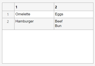
Table UI component with two rows of data. One table cell has the words "Beef" and "Bun" on separate lines, and the table row is taller so that both lines of text are visible.

UI Components: Interact with UI components using keyboard

You can use keyboard shortcuts to interact with slider, knob, and switch UI components. To move focus to a slider, knob, or switch in an app, use the Tab key. Once a component is in focus, use the arrow keys to change the value of a slider or knob or the Space or Enter keys to toggle the value of a switch.

Additionally, interacting with table UI components in figure-based apps now uses different keyboard shortcuts. To move focus to a table in an app, use the Tab key. Once a table is in focus, use the arrow keys to navigate between different cells in the table. In previous releases, the Tab key navigated between different cells in the table.

UI Components: Replace UIControl objects with UI components

If you have an existing app created using the figure function, you can now add UI components to the app. Replacing UIControl objects with UI components is a first step for updating figure-based apps to use uifigure, which is the recommended functionality for building apps.

In addition, UI components have a larger set of configuration options than UIControl objects. For example, you can replace a UIControl push button with a Button object created using the uibutton function and then add HTML markup to the button text by setting the Interpreter property to "html".

For more information about updating figure-based apps to use UI components, see Update UIControl Objects and Callbacks.

App Designer: Package and share apps more efficiently

When you package apps from App Designer to share with others, the packaging steps are simpler and use a new interface. In addition, apps are now packaged as MLTBX files instead of MLAPPINSTALL files.

To package an App Designer app, use these steps:

  1. With the app open in App Designer, on the Designer tab, select Share > MATLAB App.

  2. Review the app information by following the steps in the Configure MATLAB App for Sharing dialog box, and then click Package.

When the packaging process completes successfully, MATLAB creates an MLTBX file with the packaged app. You can install the app by opening the MLTBX file and then access the app from the Apps tab of the MATLAB Toolstrip. Or, you can share the app with others by sharing the MLTBX file directly or uploading it to MATLAB File Exchange.

For more information, see Package Apps in App Designer.

App Designer: Access toolstrip actions and Help Center resources using search

You can now use the search box in the top-right corner of App Designer to easily access toolstrip actions and Help Center resources, such as functions, examples, and answers.

For example, to show the background grid on the App Designer canvas, type the word grid in the search box. In the list of results, select the Grid toolstrip action.
Search box containing the word grid and a list of search results including toolstrip actions, functions, and examples

Text: Larger, easier-to-read text on macOS

Text in apps has a larger, more readable default font size on macOS systems. The size is now consistent across Windows and macOS systems. Specifically, objects that have a Units or FontUnits property set to "points", "inches", or "centimeters" display about 1.33x larger than their previous size on macOS systems.

For compatibility considerations, see Text: Text and other objects specified in "points", "inches", or "centimeters" are larger on macOS.

 Functionality being removed or changed

GUIDE design environment and guide function have been removed

Errors

The GUIDE design environment and guide function have been removed. You can still run existing GUIDE apps in MATLAB, but you can no longer edit apps using the drag-and-drop GUIDE environment.

To continue working with an existing GUIDE app and to maintain its compatibility with future MATLAB releases, use one of the recommendations listed in the table.

App Development NeedsStrategy
Ongoing developmentMigrate your app to App Designer using the GUIDE to App Designer Migration Tool for MATLAB.
Occasional editingEdit your app using the existing app code file that GUIDE created.
Only runningContinue to run your GUIDE app.

For more information about maintaining and migrating apps, see GUIDE Migration Strategies.

To create new apps, use App Designer.

actxcontrol, actxcontrollist, and actxcontrolselect functions have been removed

Errors

The actxcontrol, actxcontrollist, and actxcontrolselect functions have been removed. If you call the functions, MATLAB returns an error. For app development using App Designer, update your code to use alternative functionality. For a list of functionality that you can use instead, see Recommendations for MATLAB Apps Using Java & ActiveX.

pagesetupdlg function has been removed

Errors

The pagesetupdlg function has been removed. If you call pagesetupdlg, MATLAB returns an error. Use uiprintdlg instead.

printpreview, printdlg, and exportsetupdlg functions will be removed

Warns

The printpreview, printdlg, and exportsetupdlg functions will be removed in a future release. If you call printpreview or printdlg, MATLAB issues a warning and runs the new uiprintdlg function instead. If you call exportsetupdlg, MATLAB issues a warning and runs the new uiexportdlg function instead.

To simplify the interfaces, the new dialog boxes do not include options for customizing fonts, line width, or tick values, or for setting the renderer. To control the appearance of a figure that you want to print or export, set properties of the figure and the objects in the figure before opening the dialog box.

matlab.apputil.create function will be removed

Still runs

The matlab.apputil.create function will be removed in a future release. If you call matlab.apputil.create, the function now prompts you to package your app as a toolbox. Calling the function is equivalent to selecting Add-Ons > Package Toolbox from the Home tab of the MATLAB Toolstrip.

UI Components: Some default colors for UI components have changed slightly

Behavior change

Some of the default colors of UI components and containers have changed. These changes affect the light theme colors. This table describes the changes and provides the RBG triplets and color samples to compare R2025a with the previous release.

Affected App AreaAffected Component PropertiesR2024b ColorR2025a Color
Container backgrounds
  • Color property of Figure object

  • BackgroundColor property of UI container objects such as Panel

[0.94 0.94 0.94]

Sample of light gray color, the default figure background color (R2024b)

[0.9608 0.9608 0.9608]

Sample of slightly lighter gray color, the default figure background color (R2025a)

App textFontColor property of UI component objects

[0 0 0]

Example of a label (R2024b)

[0.1294 0.1294 0.1294]

Example of a label (R2025a)

Unvisited hyperlinksFontColor property of Hyperlink object

[0 0.3984 0.7969]

Example of an unclicked hyperlink (R2024b)

[0.0667 0.4431 0.7451]

Example of an unclicked hyperlink (R2025a)

Visited hyperlinksVisitedColor property of Hyperlink object

[0.5 0 0.5]

Example of a clicked hyperlink (R2024b)

[0.5216 0.0863 0.8196]

Example of a clicked hyperlink (R2025a)

UI Components: Updated look for panels and button groups in figure-based apps

Behavior change

Panels and button groups created in figure-based apps have an updated appearance. Because of this update, certain title and border options have changed.

Panel and button group titles can appear only at the top of the container. As a result, these TitlePosition values have changes in behavior.

ValueR2024b and EarlierStarting in R2025aRecommended Value
"leftbottom"

Panel with a title in the bottom left

Panel with a title in the upper left

Update your code to use "lefttop" instead of "leftbottom" to reflect the title position.
"centerbottom"

Panel with a title in the bottom center

Panel with a title in the upper center

Update your code to use "centertop" instead of "centerbottom" to reflect the title position.
"rightbottom"

Panel with a title in the bottom right

Panel with a title in the upper right

Update your code to use "righttop" instead of "rightbottom" to reflect the title position.

Panel and button group borders always appear as a line. As a result, some BorderType values have changes in behavior. Specifying BorderType as any of the options in the table causes a warning. Additionally, the default BorderType value has changed from 'etchedin' to 'line'.

ValueR2024b and EarlierStarting in R2025aRecommended Value
"etchedin"

Panel with an etched-in border

Panel with a line border

Update your code to use "line" instead of "etchedin" to reflect the border type.
"etchedout"

Panel with an etched-out border

Panel with a line border

Update your code to use "line" instead of "etchedout" to reflect the border type.
"beveledin"

Panel with a beveled-in border

Panel with a line border

Update your code to use "line" instead of "beveledin" to reflect the border type.
"beveledout"

Panel with a beveled-out border

Panel with a line border

Update your code to use "line" instead of "beveledout" to reflect the border type.

As a result of the changes to the BorderType property, the ShadowColor property has no effect and warns if you set it. To specify the border color of a panel or a button group, use the BorderColor property instead.

The ShadowColor property no longer appears in the list returned by calling the get function on a Panel or ButtonGroup object. For more information about container properties, see Panel or ButtonGroup.

UI Components: Table Extent property returns default table UI component width and height and is not recommended

Behavior change

When you query the Extent property of a table UI component created using the uitable function, the property now always returns [0 0 300 300] in pixel units, or the equivalent value if the table is using non-pixel units. The third and fourth elements of the vector represent the default table width and height. Previously, querying Extent in a figure-based app returned a vector where the third and fourth elements represent the width and height of the rectangle outlining the table area. If you use the Extent property to specify the position of UI components in your app, the table UI component might have a different size or the layout of your app might appear shifted.

Update your code to remove references to Extent using one of these alternatives:

  • Manage your app layout using a grid layout manager created using the uigridlayout function. Specify a row height or column width of "fit" to automatically scale your app layout based on the size of the table with its data.

  • Lay out the table and other UI components by manually specifying the Position property value.

The Extent property is not recommended and no longer appears in the list returned by calling the get function on a Table object.

UI Components: InnerPosition property of tab groups returns the position excluding borders and titles

Behavior change

For apps created using the figure function, when you query the InnerPosition property of a tab group, the property returns a different value than in the previous release. In addition, if the TabLocation property is 'left' or 'bottom', when you query the Position, InnerPosition, and OuterPosition properties of a tab in the tab group, the properties might return different values than in the previous release. These changes make the property values and behaviors consistent with the properties in uifigure-based apps.

This table describes the differences in the property values between R2025a and previous releases.

PropertyR2024b and EarlierStarting in R2025a
DescriptionImageDescriptionImage
InnerPosition of a tab groupA four-element vector of the form [left bottom width height] that represents the size and location of the tab group relative to the drawable area of its parent, including borders and titles of the tabs it contains

Tab group InnerPosition (blue solid line)

Tab group with tab titles on the left. A blue solid line surrounds the entire tab group, including the tab titles.

A four-element vector of the form [left bottom width height] that represents the size and location of the tab group relative to the drawable area of its parent, excluding borders and titles of the tabs it contains

Tab group InnerPosition (blue solid line)

Tab group with tab titles on the left. A blue solid line surrounds the area of the tab group that excludes the tab titles.

Position, InnerPosition, and OuterPosition of a tabA four-element vector of the form [left bottom width height] that represents the size and location of the tab relative to the tab group drawable area, where the tab group drawable area includes borders and titles

Tab Position (orange dashed line) relative to tab group drawable area (blue solid line)

Tab group with tab titles on the left. A blue solid line surrounds the entire tab group, including the tab titles. An orange dashed line surrounds the area of the tab group that excludes the tab titles, and is offset on the left from the blue solid line.

A four-element vector of the form [left bottom width height] that represents the size and location of the tab relative to the tab group drawable area, where the tab group drawable area excludes borders and titles

Tab Position (orange dashed line) relative to tab group drawable area (blue solid line)

Tab group with tab titles on the left. A blue solid line and an orange dashed line both surround the area of the tab group that excludes the tab titles.

If you notice changes in your app layout, consider updating your code in this way:

  • Tab group InnerPosition — Replace references to the tab group InnerPosition property with the tab group Position property to use the size and location of the tab group including the borders and tab titles.

  • Tab Position, InnerPosition, and OuterPosition — Replace references to the first two elements of the position vector to instead use the space taken up on the left or bottom by the tab titles. For example, if your app contains a tab group with a TabLocation value of 'left' and you reference the Position property of a tab in that tab group, replace that reference with the horizontal distance between the tab group border and the tab drawable area.

For more information about tab group and tab properties, see TabGroup and Tab.

UI Controls: Some control font size and text content might appear differently in figure-based apps

Behavior change

Controls created using the uicontrol function have these differences:

  • The default font used by the uicontrol function might have a different appearance and require a different amount of space than in previous releases. To update your app, use the Position property of the UIControl object to account for the space the text needs.

  • UIControl check boxes and tooltips do not render HTML content.

  • Radio button and toggle button callback functions are executed only when selecting a button that is not already selected. Previously, the callbacks were executed even if an app user clicked a button that was already selected.

Figures: Figure windows display a toolstrip instead of a menu bar and toolbar

Behavior change

Starting in R2025a, when you create a figure using the figure function or load a saved figure, the figure appears with a toolstrip instead of a menu bar and toolbar. The figure toolstrip provides improved options for interacting with plots and data in a figure.

However, apps and saved figures that modify the figure menu bar or toolbar (for example, by setting the ToolBar property of the Figure object) continue to display the menu bar and toolbar instead of the toolstrip. If your app relies on menu bar or toolbar functionality, you can specify that the app display the menu bar or toolbar instead of the toolstrip by setting the figure MenuBar or ToolBar properties when you create the figure for your app.

f = figure;
f.MenuBar = "figure";
f.ToolBar = "figure";

In addition, figures created from a packaged standalone desktop application and figures created when running code noninteractively using the -batch startup option continue to display the menu bar and toolbar instead of the toolstrip.

Figures: Scroll event data for WindowScrollWheelFcn figure callback returns updated scroll count values

Behavior change

When you specify a WindowScrollWheelFcn callback function for a figure created using the figure function, the callback event data returns different values in some cases. This table describes the differences.

Event Data PropertyR2024b and EarlierStarting in R2025a
VerticalScrollCount

A positive or negative number that indicates the direction and number of scroll wheel clicks. Scrolling down returns a positive value. Scrolling up returns a negative value.

The vertical scroll count is the sum of all scroll wheel clicks that occurred since the last time the callback executed. Typically, the value is 1 or -1. However, the scroll count can have a larger magnitude if the WindowScrollWheelFcn callback takes a long time to return or if the user spins the scroll wheel very fast.

A positive or negative number that indicates the direction of scrolling. Scrolling down returns 1. Scrolling up returns -1.
VerticalScrollAmountThe number of lines scrolled for each click of the scroll wheel. Typically, the value is 3, but some systems might return a different value depending on how the mouse is configured.3

Figures: Modal figures always block all MATLAB windows

Behavior change

When you create a modal figure by specifying the figure WindowStyle property as "modal", the figure window blocks interaction with all MATLAB windows, including other figure windows and the MATLAB desktop. In previous releases, modal figures created using the uifigure function did not block the MATLAB desktop.

If you need to interact with the MATLAB desktop while a modal figure is in focus, press Ctrl+C. This action causes the figure WindowStyle property to change from 'modal' to 'normal'.

Figures: Axes and containers laid out using nondefault units might appear in different positions

Behavior change

If you create a figure using the figure function and add axes or containers to the figure using a nondefault value for the Units property, the axes or containers might appear with a different location or size than in previous releases. The reason for the behavior change is that querying the Position property of a Figure object might not return the final size of the figure immediately after the figure is created.

For example, this code might create the axes at a larger size than in previous releases, and the axes width and height might be larger than half the final figure width and height.

f = figure;​
a = axes(f, ...
    Units="pixels", ...
    Position=[1 1 f.Position(3)/2 f.Position(4)/2]);​

To lay out graphics objects or UI components relative to the size of the figure they are in, use one of these strategies:

  • Use the default units to lay out the object (for example, "normalized" for Axes objects).

  • Specify the figure position using the Position property.

  • Use a layout manager by calling tiledlayout for plots or uigridlayout for UI components and containers.

Fonts: MATLAB supports slightly different set of fonts

Behavior change

The set of fonts that MATLAB can display is slightly different than in previous releases. If you specify a font that MATLAB cannot display, MATLAB instead displays the text using a common font available on the machine. If MATLAB cannot display a specified font, you can select a different font instead. To see a list of fonts installed on your system, use the listfonts function.

Text: Text and other objects specified in "points", "inches", or "centimeters" are larger on macOS

Behavior change

Objects that have a Units or FontUnits property set to "points", "inches", or "centimeters" now use a conversion value of 1 pixel = 1/96 inch on macOS systems. Previously, the conversion value was 1 pixel = 1/72 inch. As a result, these objects have increased in size by a factor of 96/72 (about 1.33x). The new size provides consistency between macOS and Windows systems.

If you have code that uses pixel units for positioning objects such UI components in App Designer or in apps created using the uifigure function, those objects are unaffected by this change. However, text objects such as titles and labels, text in axes, and text in UIControl objects appear larger by default on macOS systems. To preserve the sizes of text and other affected objects so that they match the sizes on macOS systems in previous releases, make these changes in your code:

  • Objects with Units or FontUnits set to "points" — Update the value of the property from "points" to "pixels".

  • Objects with Units or FontUnits set to "inches" — Update the value of the property from "inches" to "pixels" and multiply all Position values by 72.

  • Objects with Units or FontUnits set to "centimeters" — Update the value of the property from "centimeters" to "pixels" and multiply all Position values by 72/2.54.

Some javacomponent functionality has been removed

Behavior change

The undocumented javacomponent function has some changes in behavior and some functionality has been removed. Replace calls to the javacomponent function with documented UI component alternatives.

For more details and a list of documented functionality that you can use instead, see Recommendations for MATLAB Apps Using Java & ActiveX.

Performance

datetime Format Parsing: Improved performance when parsing common date and time formats

datetime format parsing performance is significantly faster for common date and time formats. Most date and time formats that are composed of letter identifiers separated by common delimiters see improved performance.

  • Letter identifiers specify format components such as date fields, time fields, and time zone offsets. For a list of identifiers, see the datetime Format property.

  • Common delimiters are ":", ";", ",", ".", "-", "/", and the space character.

Examples of common input formats are:

  • "dd.MM.uuuu"

  • "MM/dd/uuuu"

  • "uuuu MM dd"

  • "HH:mm, dd MMMM uuuu Z"

  • "uuuu MMM dd HH:mm:ss.SSS a ZZZZZ"

  • "uuuu-MM-dd'T'HH:mm"

  • "QQQ/uuuu"

In R2025a, there is no improvement for input formats that include D, G, Q, QQ, W, y, yy, and z. (Only the identifiers listed in the previous sentence are affected. There can still be a performance improvement when you use identifiers such as QQQ or yyyy.)

Code that uses the datetime function to parse and convert text is generally about 4–17x faster, depending on the size and format of the input array. For example, this code shows an example of the parsing performance improvement. It creates a string array of dates that use periods as delimiters. The dates in the string array use the dd.MM.uuuu format. Then the code uses the datetime function to parse and convert the string array. The code is about 9.6x faster than in the previous release.

function timingTest

s = randi([1,31],1e6,1) + ".10.2024";

d = datetime(s,InputFormat="dd.MM.uuuu");

end

The approximate execution times are:

R2024b: 3.27 s

R2025a: 0.34 s

The code was timed on a Windows 11, AMD EPYC 74F3 24-Core Processor @ 3.19 GHz test system using the timeit function.

timeit(@timingTest)

String Operations: Improved performance with small string arrays

String operations, such as string construction and indexing, show improved performance when working on small string arrays. For example, this code constructs a string from a character vector. The code is about 2x faster than in previous release.

function timingTest
for i = 1:1e7
    str = string('MATLAB');
end
end

The approximate execution times are:

R2024b: 2.4 s

R2025a: 1.2 s

As another example, this code assigns a single element of a string array. The code is about 16x faster than in the previous release.

function timingTest
str = ["MATLAB"; "Simulink"];
for i = 1:1e7
    str(1) = "MATLAB";
end
end

The approximate execution times are:

R2024b: 4.5 s

R2025a: 0.28 s

The code was timed on a Windows 11, AMD EPYC 74F3 24-Core Processor @ 3.19 GHz test system using the timeit function.

timeit(@timingTest)

writetable, writetimetable, writematrix, and writecell Functions: Improved performance when writing to existing sheets or writing new sheets with sheet names

The writetable, writetimetable, writematrix, and writecell functions show improved performance when writing data to existing sheets in XLSX, XLSM, XLTX, and XLTM files. These functions also show improved performance when writing data to new sheets with sheet names in those file types. The performance improvement increases with the number of sheets written.

For example, create an XLSX file with four sheets, where only the last sheet is nonempty.

function setupData
t1 = table(0);
filename = "test4.xlsx";
writetable(t1,filename,Sheet=4);
end

Then write data to the four individual sheets. This code is about 1.9x faster than in the previous release.

function timingTest
for ii = 1:4
    t2 = table(magic(20));
    writetable(t2,"test4.xlsx",Sheet=ii);
end
end

The approximate execution times are:

R2024b: 0.063 s

R2025a: 0.033 s

The code was timed using the timeit function.

setupData;
timeit(@timingTest)

As another example, write data to new sheets of an XLSX file, including sheet names. This code is about 1.8x faster than in the previous release.

data = rand(1000,100);
t = array2table(data);
filename = "test10.xlsx";
tic
for idx = 1:10    
    sheetname = sprintf('Sheet_%02d',idx); 
    writetable(t,filename,Sheet=sheetname);
end
toc

The approximate execution times are:

R2024b: 34.64 s

R2025a: 19.05 s

The code was timed on a Windows 11, AMD EPYC 74F3 24-Core Processor @ 3.19 GHz test system.

parquetread Function: Improved performance when reading repeated string values

The parquetread function shows improved performance when reading data containing repeated string values. For example, create a table with repeated string values, and then export the table to a Parquet file.

function setupData
rng(1)
causes = ["attack" "earthquake" "energy emergency" ...
          "equipment fault" "fire" ...
          "severe storm" "thunderstorm" "unknown" ...
          "wind" "winter storm"];
idx = randi(numel(causes),[1e7 1]);
causes = causes(idx)';
T = table(causes,VariableNames="OutageCause");
parquetwrite("causes.parquet",T);
end

Read the Parquet file. This code is about 4.8x faster than in the previous release.

function timingTest
parquetread("causes.parquet");
end

The approximate execution times are:

R2024b: 3.71 s

R2025a: 0.76 s

The code was timed on a Windows 11, AMD EPYC 74F3 24-Core Processor @ 3.19 GHz test system using the timeit function.

setupData;
timeit(@timingTest)

nufft Function: Improved performance with nonuniform sample points or query points

The nufft function shows improved performance when operating on either nonuniformly spaced sample points or nonuniformly spaced query points.

For example, this code computes the nonuniform discrete Fourier transform of a signal using 1,000,000 nonuniform sample points and 10,000 uniform query points. The code is about 13x faster than in the previous release.

function t = timingNonuniformSamplePoints
t = sort(randn(1,1e6));
f = 1:1e4;
x = randn(size(t));

y = @() nufft(x,t,f);
t = timeit(y);
end

The approximate execution times are:

R2024b: 1.59 s

R2025a: 0.12 s

As another example, this code computes the nonuniform discrete Fourier transform of a signal using 1,000,000 uniform sample points and 10,000 nonuniform query points. The code is about 14x faster than in the previous release.

function t = timingNonuniformQueryPoints
t = 1:1e6;
f = sort(randn(1,1e4));
x = randn(size(t));

y = @() nufft(x,t,f);
t = timeit(y);
end

The approximate execution times are:

R2024b: 0.97 s

R2025a: 0.07 s

The code was timed on a Windows 11, AMD EPYC 74F3 24-Core Processor @ 3.19 GHz test system by calling the timingNonuniformSamplePoints and timingNonuniformQueryPoints functions.

mink, maxk, and topkrows Functions: Improved performance when returning a large number of rows for numeric or logical data

The mink, maxk, and topkrows functions show improved performance for numeric data, including complex data, and logical data when the number of rows to return is large.

  • The mink and maxk functions show improved performance when k (the number of minima or maxima to return) is at least 512 and is at least 8% of the operating dimension length.

  • The topkrows function shows improved performance when k (the number of rows to return) is at least 2048 and is at least 20% of the total number of rows.

For example, this code returns the smallest 5000 elements of each column in a numeric matrix containing 10,000 rows by using the mink function. The code is about 3.75x faster than in the previous release.

function timingTestMink
A = rand(1e4,10);
for i = 1:120
    M = mink(A,5000);
end
end

The approximate execution times are:

R2024b: 1.05 s

R2025a: 0.28 s

Similarly, this code returns the top 5000 rows from a numeric matrix containing 10,000 rows in descending order, primarily based on the first column, by using the topkrows function. The code is about 2x faster than in the previous release.

function timingTestTopkrows
A = rand(1e4,10);
for i = 1:120
    T = topkrows(A,5000);
end
end

The approximate execution times are:

R2024b: 0.14 s

R2025a: 0.07 s

In both cases, the code was timed on a Windows 11, AMD EPYC 74F3 24-Core Processor @ 3.19 GHz test system using the timeit function.

timeit(@timingTestMink)
timeit(@timingTestTopkrows)

fillmissing Function: Improved performance when filling entries using linear interpolation

The fillmissing function shows improved performance when you specify the fill method as "linear".

For example, this code uses linear interpolation to replace the NaN values in a 1000-element numeric vector. The code is about 2.2x faster than in the previous release.

function timingTest
A = rand(1000,1);
idx = randperm(1000,50);
A(idx) = NaN;
for i = 1:2e4
    F = fillmissing(A,"linear");
end
end

The approximate execution times are:

R2024b: 0.84 s

R2025a: 0.38 s

The code was timed on a Windows 11, AMD EPYC 74F3 24-Core Processor @ 3.19 GHz test system using the timeit function.

timeit(@timingTest)

groupsummary Function: Improved performance when applying multiple computation methods

The groupsummary function shows improved performance when you specify at least two of the "sum", "mean", "min", or "max" computation methods, especially when the number of data points per group is small.

For example, this code computes the sum and maximum for a table with one data variable and one grouping variable. The code is about 6.6x faster than in the previous release.

function timingTest
data = rand(1000,1);
groups = categorical(randi(500,[1000 1]));
for i = 1:1200
   groupsummary(data,groups,["sum" "max"]);
end
end

The approximate execution times are:

R2024b: 2.11 s

R2025a: 0.32 s

The code was timed on a Windows 11, AMD EPYC 74F3 24-Core Processor @ 3.19 GHz test system using the timeit function.

timeit(@timingTest)

uifigure Function: Improved performance when creating UI figure

Creating a figure using the uifigure function has improved performance. This improvement affects App Designer apps because App Designer uses the uifigure function to create the figure for an app. The performance improvement is most noticeable when you create a single figure outside of a loop.

For example, create a single UI figure. This code is about 5.7x faster than in the previous release.

function timingFigure
tic
f = uifigure;
drawnow
toc
end

The approximate execution times are:

R2024b: 2.0 s

R2025a: 0.35 s

The code was timed on a Windows 11, Intel Xeon CPU W-2133 @ 3.60 GHz test system by calling the timingFigure function.

Property Inspector: Improved performance when opening for the first time

The Property Inspector shows improved performance when opening for the first time in a MATLAB session. The delay between clicking More Properties or calling inspect and the Property Inspector being ready is reduced.

For example, open the Property Inspector for the first time in a MATLAB session. You can use the Property Inspector about 2.3x sooner than in the previous release.

axes
tic
inspect
toc

The approximate execution times are:

R2024b: 4.65 s

R2025a: 2.00 s

The code was timed on a Windows 11, AMD EPYC 74F3 24-Core Processor @ 3.19 GHz test system.

Axes Toolbar: Improved performance for single Cartesian axes when opening for the first time

The axes toolbar shows improved performance for a single set of Cartesian axes when opening for the first time in a MATLAB session. The delay between pausing on the axes and the axes toolbar being visible is reduced.

For example, create a set of Cartesian axes by using the axes command. When you pause on the set of axes for the first time in a MATLAB session, the axes toolbar becomes visible about 2x faster than in the previous release.

The approximate rendering times are:

R2024b: 1.8 s

R2025a: 0.9 s

The interaction was timed on a Windows 11, AMD EPYC 74F3 24-Core Processor @ 3.19 GHz test system by pausing on a set of Cartesian axes.

Plot Interactions: Improved responsiveness when interacting with scatter plots that have circle markers

Scatter plots that display circle markers show improved responsiveness when you perform interactions, such as panning, zooming, and rotating. The improvement is more noticeable when you plot more than 25,000 points and your system has a GPU.

For example, on a Windows 11, Intel Xeon CPU W-2133 @ 3.60 GHz test system that has an NVIDIA Quadro® P600 GPU, if you run this code and then drag to rotate the plot, the rotation is smoother and follows your cursor more closely in R2025a than in the previous release.

f = figure;
ax = axes(f);
x = randn(1,2000000);
y = randn(1,2000000);
z = randn(1,2000000);
scatter3(ax,x,y,z,"filled")
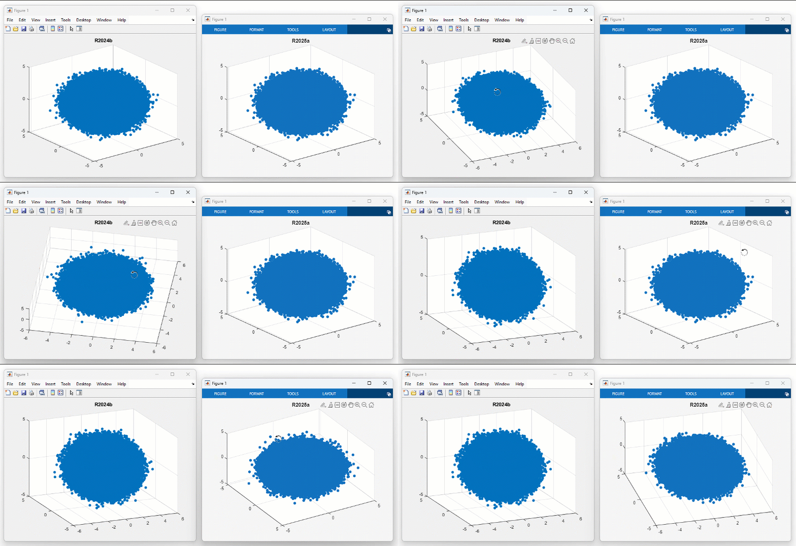
Animation of a rotating 3-D scatter plot in R2024b and R2025a

Plot Interactions: Improved responsiveness when panning or zooming within line plots

Line plots in apps or in figures created with the uifigure function show improved responsiveness when you pan or zoom within the axes. If you plot a large number of points and then pan within the axes, the content that was previously outside the boundaries of the axes comes into view more quickly in R2025a than in the previous release. Before R2025a, gaps in the content appeared as you panned or zoomed.

For example, on a Windows 11, Intel Xeon CPU W-2133 @ 3.60 GHz test system, if you run this code and then pan within the axes, the content updates immediately without any gaps.

f = uifigure;
ax = axes(f);
x = 1:250000;
y = [log(x') log(x')+2 log(x')+4] + rand(250000,1);
plot(ax,x,y)
xlim(ax,[1500 4500])
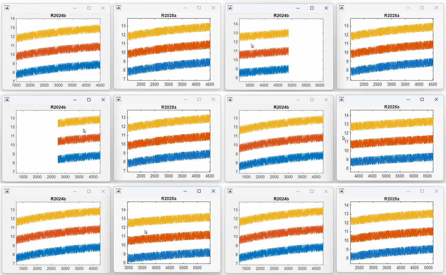
Animation of panning within a plot in R2024b and R2025a

If you create the figure with the figure function, the content that was previously outside the boundaries of the axes comes into view quickly (as in the previous release), but the interaction follows the cursor more closely.

Animations in Apps and MATLAB Online: Improved performance for animations in loops

Animations that involve updating plot data in a loop and using the drawnow command show improved performance. You can observe the improvement if you run the animations in any of these contexts:

  • In an app created in App Designer

  • In a figure created with the uifigure function

  • In any type of figure created in MATLAB Online

For example, create a figure using the uifigure function and display a line animation. This code is about 5.2x faster than in the previous release.

f = uifigure;
ax = axes(f);
p = animatedline(ax);
xlim(ax,[0 10])
ylim(ax,[-1 1])
x = linspace(0,10,500);
drawnow 
tic
for i = 1:500
  y = sin(x);
  addpoints(p,x(i),y(i))
  % Redraw figure after adding a point
  drawnow
end
toc

The approximate execution times are:

R2024b: 15.61 s

R2025a: 2.98 s

The code was timed on a Windows 11, Intel Xeon CPU W-2133 @ 3.60 GHz test system.

Plots in Apps: Improved performance when creating multiple legends

Creating multiple legends in an app created in App Designer or using the uifigure function shows improved performance. For example, create 16 plots in a 4-by-4 tiled chart layout and add a legend to each plot in a separate loop. This code is about 1.7x faster than in the previous release.

f = uifigure;
% Create 16 plots in a 4-by-4 tiled chart layout
t = tiledlayout(f,4,4);
for i = 1:16
    ax = nexttile(t);
    plot(ax,magic(10));
end
drawnow
tic
for i = 1:16
    % Create legend in the ith axes
    legend(nexttile(t,i))
    drawnow
end
toc

The approximate execution times are:

R2024b: 9.45 s

R2025a: 5.66 s

The code was timed on a Windows 11, Intel Xeon CPU W-2133 @ 3.60 GHz test system.

Operations on Windows 11 Platforms with Multiple Processor Groups: Improved performance

On machines running Windows 11 (or later) or Windows Server 2022 (or later) with multiple processor groups, MATLAB can now use cores across all existing processor groups. Previously, MATLAB used only the cores in the processor group running MATLAB. Because of this change, computationally expensive operations can show improved performance.

For example, this code performs matrix multiplication with two 15,000-by-15,000 matrices. The code is about 1.6x faster than in the previous release.

function t = timingTest
A = ones(15000);
B = ones(15000);

f = @() A*B;
t = timeit(f);
end

The approximate execution times are:

R2024b: 5.40 s

R2025a: 3.42 s

The code was timed on a Windows 11, AMD Ryzen™ Threadripper™ PRO 7995WX 96-Core Processor @ 2.5 GHz test system by calling the timingTest function. On this test system, the default maximum number of computational threads in R2024b is 64, while the default maximum number of computational threads in R2025a is 96.

Software Development Tools

 Project Panel: Manage project environment and view issues using improved interface

Starting in R2025a, the project user interface is located in the Project panel, where you can access simplified workflows and new features.

This table describes how to perform common project tasks.

TaskR2024b and EarlierStarting in R2025a
Create a project from an existing folder.On the Home tab, select New > Project > From Folder.On the Home tab, select New > Project. Then, select an existing folder. If the folder you select is empty, the software creates a blank project.
Create an empty project.On the Home tab, select New > Project > Blank Project.
Clone or check out a remote repository and create a project in the working copy.On the Home tab, select New > Project > From Git or From SVN.

To create a project from a non-project source control repository:

  1. On the Home tab, select New > Git Clone or SVN Checkout.

  2. Create a project from an existing working folder. On the Home tab, select New > Project.

Create a project from a Simulink template.On the Home tab, select New > Project > From Simulink Template.Use the Simulink Start Page to create a project from a Simulink template. For more information, see Create New Project Using Templates (Simulink).
Add files to a project.On the Project tab, in the Tools gallery, click Add Files.In the Project panel, right-click a file or a folder and select Add to Project or Add Folder to Project (Including Contents).
Check for project files with unsaved changes.On the Project tab, in the Tools gallery, click Show Unsaved Changes.On the Project tab, in the Environment section, select Project Issues > Unsaved Changes.
Run project checks.On the Project tab, in the Tools gallery, click Check Project.On the Project tab, in the Environment section, click Project Issues. In the Checks tab of the Project Issues panel, click Run Checks.
Share project by email.On the Project tab, in the File section, select Share > Email.

On the Project tab, in the File section, select Share > Archive. Then, attach the project archive to an email.

For more ways to share projects, see Share Projects.

Project References: Componentize large projects with improved usability

Organize a project into smaller projects with improved usability. Improvements to referenced projects workflows include:

  • Accessing shortcuts in all referenced projects from the top-level project

  • Automatic updates when renaming, deleting, or removing files in the entire project hierarchy

  • Identifying issues in your project hierarchy, such as circular or missing dependencies

  • Support for moving files and folders between projects in the same project hierarchy

For more information, see Componentize Large Projects.

Project Comparison: Compare MATLAB projects

Starting in R2025a, when you compare folders, MATLAB detects whether they are project root folders. MATLAB looks for and compares the project definition files stored in the resources folder. Project definition files contain information about the project path, project settings, shortcuts, labels, and referenced projects. For more information, see Compare MATLAB Projects.

Dependency Analyzer: View project hierarchy and issues

You can use the Project Hierarchy view in the Dependency Analyzer to visualize the relationships between the top-level project and the referenced projects. The hierarchy graph also flags issues about missing projects and circular dependencies. For more information, see Explore the Dependency Graph, Views, and Filters.

Dependency Analyzer: Analyze dependencies in referenced projects

You can now enable dependency analysis inside referenced projects. To specify the scope of the analysis to include referenced projects, in the Dependency Analyzer toolstrip, select Analyze > Referenced Projects. For more information, see Dependency Analyzer Scope and Limitations.

Project API: List issues on project startup and shutdown

You can list all issues that occur when a project opens and closes using the listStartupIssues and listShutdownIssues functions.

Project API: Add all folders and files to project

You can now programmatically add all folders, subfolders, and files to a project in one step using the addFolderIncludingChildFiles function.

Project API: Analyze file dependencies in referenced projects

You can now include files in project references when you run a dependency analysis using the listImpactedFiles, listRequiredFiles, and updateDependencies functions.

Project API: Process multiple project files simultaneously

Starting in R2025a, project functions support processing multiple files, folders, labels, and categories in one function call. This change reduces the need to make multiple function calls and create for-loops.

For example, this table shows how to update your code to add multiple files to a project at once.

R2024b and EarlierStarting in R2025a
proj = currentProject;
Files = ["File1","File2","File3"];
for i = 1:length(Files)
   addFile(proj,Files{i});
end
proj = currentProject;
Files = ["File1","File2","File3"];
addFile(proj,Files);

The functions that support bulk processing are: addFile, addFolderIncludingChildFiles, removeFile, addPath, removePath, addStartupFile, removeStartupFile, addShutdownFile, removeShutdownFile, addShortcut, removeShortcut, createLabel, addLabel, findLabel, removeLabel, createCategory, findCategory, and removeCategory.

Project API: Improved performance when interacting with project programmatically

When you interact with a MATLAB project programmatically, the project functions and operations perform significantly faster. For example, this code saves the path of 731 project files in a variable. The code is about 7.3x faster than in the previous release.

function timingTest
  proj = currentProject;
  allProjectFiles = proj.Files;
  filesPath = [allProjectFiles.Path];
end

The approximate execution times are:

R2024b: 0.921 s

R2025a: 0.126 s

The code was timed on a Windows 11, AMD EPYC 9474F 48-Core Processor @ 3.60 GHz test system using the timeit function.

timeit(@timingTest)

Code Analyzer: Configure Custom Naming Conventions for MATLAB Identifiers

Configure the Code Analyzer to display a custom check when MATLAB identifiers do not adhere to specified naming conventions. For more information on configuring custom Code Analyzer checks, see Configure Code Analyzer.

You can configure required or disallowed prefixes and suffixes for identifiers. A message will be displayed if an identifier does not follow the naming convention. Specified phrases can be disallowed and a message will be displayed if they are found anywhere in the identifier name. For example, you could require that property names start with the prefix prop or property.

"naming": {
        "property" : {
            "requiredPrefix" : ["prop","property"]
        }
}

You can configure casing so that identifiers conform to one or more casing standards by specifying a "casing" property containing a string array where each element is a casing standard. If more than one casing is specified, then identifiers must satisfy at least one specified casing. For example, you could require that function names use lowerCamelCase and classes use UpperCamelCase.

"naming": {
        "function" : {
            "casing" : "lowerCamelCase"
        },
        "class" : {
            "casing" : "UpperCamelCase"
        }
}

You can create a custom naming convention check by specifying a regular expression. A message will be displayed if the identifier name does not fully match the specified regular expression. Required prefixes and suffixes are not excluded from this check. Each identifier type can have only a single regular expression check. For example, you could require that variable names use only lowercase letters.

"naming": {
        "variable" : {
            "regularExpression" : "^([a-z]+)$"
        }
}

 Source Control Panel: Work with multiple folders and projects under Git and SVN source control

Use the Source Control panel to interact with folders and projects under Git and SVN source control, manage modified and untracked files, and perform source control operations. If the Source Control icon is not in the sidebar, click the Open more panels button and select the Source Control panel.

The Source Control panel shows two working folders, one under SVN and the other one under Git source control.

For more information, see Source Control Integration in MATLAB.

Source Control: Check for unsaved files before commit

Starting in R2025a, you can configure MATLAB to prompt you about unsaved changes before performing source control actions such as commit, merge, SVN update, and Git branch switch. On the Home tab, in the Environment section, click Settings. Select MATLAB > Source Control. Then, select Check for unsaved files before source control operations.

Git Source Control: View line-by-line revision history for entire MATLAB file

You can view the line-by-line revision history for an entire MATLAB file under Git source control using Blame View directly within MATLAB. For more information, see Annotate Lines in MATLAB Editor Using Git History.

Git Source Control: Create shallow clone of Git repository

You can perform a shallow clone by specifying the number of the latest commits you want to clone. For more information, see Clone Git Repository in MATLAB.

Git Source Control: Share local repository to GitHub

You can share a local Git repository to GitHub directly within MATLAB. For more information, see Share Git Repository to Remote.

Git Source Control: Ignore files interactively

You can add files and folders to the .gitignore file interactively from within MATLAB. For more information, see Create Local Git Repository in MATLAB.

Git Source Control: Cherry-pick or squash Git commits, and rebase Git branches

Starting in R2025a, the MATLAB Git integration supports these workflows:

Git Source Control: Create, merge, and manage Git branches and remotes with improved usability

For folders and projects under Git source control, you can use the Branch Manager to manage multiple local and remote repositories, find and compare commits, and create, delete, and merge branches.

Git Source Control: Work with submodules in MATLAB with improved usability

You can work with and manage multiple Git repositories at a time using the Source Control panel and the Branch Manager. Starting in R2025a, when you pull changes in the main repository, MATLAB updates the submodules recursively. For more information, see Work with Git Submodules in MATLAB.

Git Source Control: Check out Git branch to separate folder using worktrees in MATLAB

You can check out a branch to a separate folder using Git worktrees directly within MATLAB. For more information, see Create and Manage Git Worktrees.

Git Source Control: Use avatars and verify commit signatures in MATLAB

Starting in R2025a, you can enable MATLAB to generate local avatars or retrieve globally recognized avatars from the web.

When you enable commit signing, MATLAB now verifies commit signatures. A green verification icon appears next to your avatar and username in both the Branch Manager and the line annotations in the MATLAB Editor.
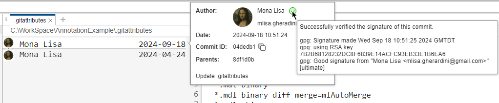
Avatar and verification icon in the line annotation of a file in the MATLAB Editor

For more information, see Configure Git Settings.

Git Source Control: MATLAB supports Git LFS process filter

Starting in R2025a, if you configure a process for an LFS filter, MATLAB launches and communicates with the process for multiple files at the same time, rather than running a new process for every file separately. This speeds up source control actions in MATLAB, such as adding files, committing files, and getting file statuses.

To configure a process for the LFS filter, install Git LFS and run !git lfs install. For more information, see Configure Git to Use Git LFS.

Installing Git LFS defines this information in the .gitconfig file.

[filter "lfs"]
	clean = git-lfs clean -- %f
	smudge = git-lfs smudge -- %f
	process = git-lfs filter-process
	required = true

Git API: List modified files between commits or branches and save file revisions to disk

Starting in R2025a, the MATLAB Git integration supports more continuous integration workflows:

  • List the modified files between two Git commits or branches using the diffCommits function.

  • Save a Git revision of a file to disk using the saveFileRevision function.

Git API: Add and remove remotes

You can add a remote to a Git repository using the addRemote function. To delete a remote, use the removeRemote function.

SVN Source Control: Remember credentials for SVN repositories

Starting in R2025a, MATLAB SVN integration remembers usernames and tokens when you interact with SVN repositories. To adjust or disable credential management, use the SVN source control settings. For more information, see Configure SVN Settings.

Comparison and Merge Tools: View tag and branch details for files under source control

Starting in R2025a, when you compare or merge files under source control, the comparison and merge tools include source control information such as the branch name and tags in the file details.
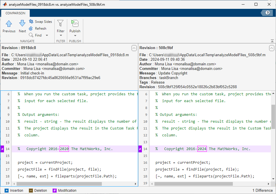
Comparison report showing details for compared files such as tags and branches.

Build Automation: Create custom reusable tasks

You can create custom task classes by subclassing the matlab.buildtool.Task class and specifying task actions, inputs, and outputs using the TaskAction, TaskInput, and TaskOutput attributes. For more information, see Create Custom Reusable Tasks.

Build Automation: Run tasks interactively from Editor or MATLAB project

If your build file named buildfile.m is open in the MATLAB Editor or if your MATLAB project contains a build file named buildfile.m in its root folder, then you can interactively run the default tasks or a specific task in the build file from the MATLAB Toolstrip. You can also customize your build run by selecting build options from the toolstrip. For more information, see Run Build from Toolstrip.

 Build Automation: Expanded support for MATLAB projects

The build tool provides expanded support for MATLAB projects. If your build file is in a MATLAB project folder, including any subfolder:

  • The matlab.buildtool.Plan.load method opens the project if it is not open.

  • The buildtool command and the run method open the project if it is not open. In previous releases, they open the project only if the build file is in the project root folder.

  • The Project property of the matlab.buildtool.Plan class provides programmatic access to the project.

 Compatibility Considerations

Starting in R2025a, the buildtool command opens the project before running the main function of the build file and leaves the project open after running the build. In previous releases, the command opens the project after running the main function of the build file and closes the project after running the build.

Build Automation: Display why tasks run

If you specify the -verbosity option of the buildtool command to display build output at the matlab.automation.Verbosity.Detailed level or above, then the build tool includes the reason for running each task. For instance, when rerunning a task in an incremental build, the build tool displays a summary of changes to the inputs and outputs of the task since its last successful run. For an example, see Create and Run Tasks with Inputs and Outputs.

Build Automation: Create group of MexTask instances using forEachFile static method

You can create a group of tasks that build MEX files by using the new matlab.buildtool.tasks.MexTask.forEachFile method.

Build Automation: Filter test suite using selectors

You can select a subset of tests to run by using the Selector property of the matlab.buildtool.tasks.TestTask class. For example, create a task that runs the tests in the feature1 subfolder of your current folder that have the "Unit" tag.

import matlab.buildtool.tasks.TestTask
import matlab.unittest.selectors.*

task = TestTask(Selector= ...
    HasBaseFolder(fullfile(pwd,"feature1")) & HasTag("Unit"));

Unit Testing Framework: Rerun tests from most recent test run using Test Browser

You can rerun the tests from your most recent test run using the Test Browser app. Click the drop-down arrow to the right of the Run current suite button on the toolbar and then select Rerun Tests.

Unit Testing Framework: Identify most recent test results in Test Browser

You can distinguish the test results produced in the most recent test run from those produced in earlier test runs. In the Test Browser panel, the statuses of tests that ran before the most recent test run appear dimmed, allowing you to identify and manage outdated test data. For an example, see Run Parameterized Tests.

Unit Testing Framework: Control whether to use Test Browser from toolstrip

When you run a function-based or class-based test file using the Run Tests section on the toolstrip, you can control whether to run the tests and display results using the Test Browser app. To access this test option, with your test file open, on the Editor or Live Editor tab, select Run Tests > Customize Test Run, and then select or clear the Use Test Browser option.

If you choose not to use the test browser by clearing the Use Test Browser option, then your tests run in the Command Window instead. Your selection persists across MATLAB sessions.

Unit Testing Framework: Create default test runner using withDefaultPlugins static method

You can use the new matlab.unittest.TestRunner.withDefaultPlugins method to create a test runner configured with default plugins. These plugins are used by the testing framework by default when running tests.

 Toolbox Packaging: Create and package toolboxes using projects

Starting in R2025a, toolbox packaging is integrated with projects. You can use tasks within a project to configure and package your toolbox.

To package your toolbox files, create a project from the folder containing your files. Then, with the project open, go to the Project tab, and in the Tools section, click Package Toolbox. Configure your toolbox using the toolbox task and then click Package Toolbox at the top-right corner of the task to create your toolbox installation file.

If you have a toolbox created in a release before R2025a as well as its associated .prj file, MATLAB automatically upgrades your toolbox to the project workflow.

For more information, see Create and Share Toolboxes.

 Compatibility Considerations

In the new project workflow, toolbox image files must now be contained within the project folder. In addition, toolbox files must be contained within your selected toolbox folder.

Extension Points: Extend the MATLAB desktop using extension points

Extend various functionalities of the MATLAB desktop using extension points. For example, you can use extension points to add items to the quick access toolbar or to the Files panel context menu. To use extension points, create a JSON file named extensions.json, place it in a folder named resources, and add a set of JSON declarations to the file. Then, to enable your customizations, add the folder containing the resources folder with the extensions.json file to the MATLAB path.

For more information, see Extend MATLAB Using Extension Points.

 Functionality being removed or changed

Referenced projects no longer support checkpoints

Behavior change

You can no longer use checkpoints in referenced projects. To track changes in referenced projects and compare changes in referenced project files to a specific version, use source control instead.

gitinit automatically adds project files to source control

Behavior change

Starting in R2025a, if you use a MATLAB project to manage the files in the folder, the gitinit function automatically adds all files with the status In project to source control.

SVN commands are no longer supported via bang operator in MATLAB on Linux

Behavior change

Starting in R2025a, on Linux systems, you cannot call svn commands from within MATLAB using the bang symbol !, for example, !svn status. Use !env -i HOME="$HOME" svn status instead.

Test Browser retains tests when a specific test procedure is run from toolstrip

Behavior change

If you run a specific test procedure using the Run Current Test button on the MATLAB Toolstrip, the Test Browser app retains the tests already imported from the corresponding test file. In previous releases, the test browser removes the tests imported from the test file before running the specified test procedure.

Single Graphics task replaces 2-D and 3-D tasks in bench function

Behavior change

In the bench function, the existing 2-D and 3-D tasks have been replaced by a single Graphics benchmarking task. The new Graphics task is a better benchmark for the updated graphics system, which uses more modern architecture, and represents a wider range of graphics workflows.

This table compares the R2024b and R2025a execution times using a Windows 11 Enterprise, Intel Core i9-12900 @ 2.4GHz test system. The measured values are expressed in seconds.

TaskExecution Times of Tasks in R2024bExecution Times of Tasks in R2025a
LU0.23840.2408
FFT0.15380.1535
ODE0.08300.0858
Sparse0.21120.2090
2-D0.1485Not applicable
3-D0.2100Not applicable
GraphicsNot applicable0.1342

External Language Interfaces

Call C++ from MATLAB: Pass MATLAB structs to and from C++ functions

You can pass MATLAB structures directly to and from C++ functions. To configure a function to accept structure arguments, set MLTYPE to "struct" for input or output arguments in the library definition file. For information about configuring a C++ struct parameter, see Struct Types.

When you set the type to struct, the help for the C++ member shows the type as a struct. For example, display the help text for the MyStruct class in library libname.

help clib.libname.MyStruct
MyStruct -  clib.libname.MyStruct    Representation of C++ class MyStruct.

      struct with fields:  
      ID             5 element vector char
      amount         single
      x              double

For more information and examples, see Pass struct Parameter.

Call C++ from MATLAB: Pass environment variables in out-of-process mode

When your MATLAB interface to a C++ library uses out-of-process execution mode, you can pass system environment variables to the process hosting the interface by using the clibConfiguration function with the OutOfProcessEnvironmentVariables name-value argument. To use this argument, you must also specify the ExecutionMode name-value argument as "outofprocess".

Call C++ from MATLAB: Stop out-of-process execution using Ctrl+C

Pressing Ctrl+C during C++ library interface out-of-process execution stops the execution of a MATLAB command. For more information, see Load C++ Library In-Process or Out-of-Process.

 Call MATLAB from C++: Create and use single-precision sparse matrices

These MATLAB Data API for C++ templated classes, which already support double-precision sparse matrices, now support single-precision sparse matrices:

 Compatibility Considerations

If you save a single-precision sparse matrix to a MAT file, you can load it into an earlier release of MATLAB. However, how the data is loaded depends on the release of MATLAB:

  • MATLAB R2021b through R2024b — MATLAB warns that the data has an unsupported data type and loads it as a double-precision sparse matrix.

  • MATLAB R2021a and earlier — MATLAB loads the data as a single-precision sparse matrix, but you cannot use the matrix because its data type is unsupported. Attempting to use the matrix can result in undefined behavior.

 C MAT File API: Maximum length of variable names increased to 2048 characters

The maximum allowed identifier length defined by the macro mxMAXNAM has increased to 2048 characters. This change allows variables, functions, classes, and many other entities to have names of up to 2048 characters. Using longer identifiers might negatively impact performance and memory. Operating systems might have maximum filename lengths that are shorter than this limit.

 Compatibility Considerations

Previously, the maximum length of identifiers was 63 characters. Recompile MEX files and engine or MAT file applications that use the constant mxMAXNAM.

Call MATLAB from Python: Automatically convert between Python and MATLAB datetime and duration types

When working in Python, you can now return MATLAB datetime and duration values directly to Python. If the MATLAB datetime or duration value is scalar, MATLAB Engine API for Python automatically converts the datetime or duration value to a Python datetime.datetime or datetime.timedelta object. If you pass a MATLAB datetime or duration array to Python and the NumPy module is available in the Python environment, the MATLAB engine automatically converts the datetime or duration array to a Python numpy.datetime64 or numpy.timedelta64 array.

If you pass a Python datetime.datetime or datetime.timedelta object to MATLAB, the MATLAB engine automatically converts it to a MATLAB datetime or duration value. The engine also automatically converts Python numpy.datetime64 and numpy.timedelta64 objects and arrays to MATLAB datetime and duration values and arrays.

If the NumPy module is not available when you return a MATLAB datetime or duration array to Python, the MATLAB engine converts the array to a Python object of type matlab.object.

For more information, see How MATLAB Handles Datetime and Duration Types in Python.

Call MATLAB from Python: Automatically convert between MATLAB tables, timetables, and Python Pandas DataFrames

When working in Python, you can now return MATLAB tables or timetables directly to Python. MATLAB Engine API for Python automatically converts the table or timetable to a Python Pandas DataFrame. The MATLAB engine also automatically converts a Python Pandas DataFrame to a MATLAB table or timetable when you pass it from Python to MATLAB.

If the Python Pandas module is not available when you pass a MATLAB table or timetable to Python, the MATLAB engine converts the table or timetable to a Python object of type matlab.object.

For more information, see Use MATLAB Tables and Timetables in Python.

Call Python from MATLAB: Switch execution modes without restarting MATLAB

When working with Python in MATLAB, you can now change the execution mode of the Python interpreter from OutOfProcess to InProcess after terminating the process associated with the Python interpreter. To change the execution mode, call pyenv(ExecutionMode="InProcess"). Previously, if you wanted to change the execution mode from OutOfProcess to InProcess, you had to restart MATLAB before calling pyenv with the new version information.

For more information, see terminate.

Call .NET from MATLAB: Save .NET objects to MAT files

You can save (serialize) .NET objects to a MAT file. For more information, see Save and Load .NET Objects in MAT Files.

Call .NET from MATLAB: Select specific numerical version of .NET

For a .NET Runtime environment specified as "core", you can select a specific numerical version using the dotnetenv function Version name-value argument. Use the Frameworks name-value argument to choose a target framework. For example:

ne = dotnetenv("core",Version="8",Frameworks="Microsoft.WindowsDesktop.App");

Web Services: Keep sensitive information encrypted when using weboptions and matlab.net.http.Credentials objects

You can avoid saving credentials and other sensitive information as plain text in properties of weboptions and matlab.net.http.Credentials objects by using a secretID object. First, save sensitive information to your MATLAB vault as a secret using the setSecret function. Then when you set an object property, such as the Username and Password properties of a matlab.net.http.Credentials object, specify a secretID object to keep your sensitive information encrypted.

MATLAB Packages: Java files supported in packages

Starting in R2025a, you can add Java code to MATLAB Packages. You can specify the language of package folders by setting the languages property of the matlab.mpm.PackageFolder object. When package is installed, all Java resources in a folder designated as java are added to both the dynamic and static class path.

If the languages property of a package folder is not designated as matlab, MATLAB files in that folder are ignored. If a package folder is not designated as java, JAR files in that folder are ignored.

 Functionality being removed or changed

Python interface converts MATLAB arrays to Python NumPy arrays when passed as input to Python functions

Behavior change

When you pass a MATLAB array as input to a Python function and the NumPy module is available in the Python environment, Python Interface now automatically converts the array to a Python NumPy array.

If the NumPy module is not available when you pass a MATLAB array as input to a Python function, Python Interface now handles vector input as it does matrix input—Python Interface converts these inputs to Python memoryview objects.

Previously, when you passed a MATLAB vector to a Python function, Python Interface converted the vector to a Python array.array object.

For more information, see Pass MATLAB Data to Python.

MATLAB truncates values of unsigned integer types when passing them to C shared library function

Behavior change

Starting in R2025a, MATLAB truncates the value for unsigned integer types when you pass the value to a function in a C shared library loaded by the loadlibrary function. The behavior for unsigned integer types is now consistent with that of signed integer types. Previously, when you passed a value of an unsigned integer type and the value was out-of-range for the type, MATLAB threw an error.

Example CodeOutput in R2024b and EarlierOutput Starting in R2025a

This C code from a C library defines value as short and unsigned short types.

 struct S16 {
     short value; % -32768 to 32767
 };
 struct SU16 {
     unsigned short value; % 0 to 65535
};
 

This MATLAB code creates a short variable and assigns an out-of-range value.

mls16.value = 123456;
lps16 = libpointer('S16Ptr', mls16);
lps16.Value

MATLAB truncates the value to 32767.

ans =
  struct with fields:
     value: 32767

Same behavior as R2024b.

This MATLAB code creates an unsigned short variable and assigns an out-of-range value.

mlsu16.value = 123456;
lpsu16 = libpointer('SU16Ptr', mlsu16)

MATLAB displays an error.

Cannot convert data value for field value due to error:
Value exceeds the legal range for the data type.
Error in libpointer (line 21)
 ptr=lib.pointer(varargin{:});
     ^^^^^^^^^^^^^^^^^^^^^^^^

MATLAB truncates the value to 65535.

ans =
  struct with fields:
     value: 65535

actxcontrol, actxcontrollist, and actxcontrolselect functions have been removed

Errors

The actxcontrol, actxcontrollist, and actxcontrolselect functions have been removed. If you call the functions, MATLAB returns an error. MATLAB supports COM server objects only.

Hardware Support

Raspberry Pi Hardware: Support for 64-bit Debian 12 Bookworm and 64-bit Debian 11 Bullseye

You can now use Raspberry Pi Blockset with Raspberry Pi boards running on 64-bit Debian® 12 Bookworm and 64-bit Debian 11 Bullseye operating systems. This support is available only for the MATLAB desktop environment.

Arduino Hardware: Support for Arduino UNO R4 WiFi and Minima boards in MATLAB Online

You can now use the arduino object in MATLAB Support Package for Arduino Hardware to connect to Arduino UNO R4 WiFi and Minima boards over USB with MATLAB Online.

Arduino Hardware: Support for Servo Motors and Sensors with Arduino UNO R4 WiFi and Minima Boards

You can now use MATLAB Support Package for Arduino Hardware to interface Arduino UNO R4 WiFi and Minima boards with servo motors and sensors supported by the support package. This feature is available for both MATLAB desktop and MATLAB Online environment.

Arduino Hardware: Enhancing voltage data acquisition capabilities with readVoltage function

You can now use the readVoltage function in MATLAB Support Package for Arduino Hardware to acquire voltage data at a higher sampling rate. This function also allows you to acquire voltage data at the specified sample rate for a specific duration or number of samples, and return data in a particular output format. Starting this release, you can configure the readVoltage function using these name-value arguments: NumSamples, Duration, SampleRate, and OutputFormat.

 Functionality being removed or changed

Raspberry Pi Hardware: Support for Buster Raspberry Pi Linux operating system will be removed

Still runs

Support for the 32-bit Buster Raspberry Pi Linux operating system will be removed in a future release for Raspberry Pi Blockset in the MATLAB desktop and MATLAB Online environment. You will no longer be able to use the support package to communicate with a Raspberry Pi board that runs a Buster operating system. You must upgrade the Raspberry Pi Linux operating system to 32-bit or 64-bit Bullseye or Bookworm in the MATLAB desktop environment and 32-bit Bullseye or Bookworm in the MATLAB Online environment.

R2024b

New Features, Bug Fixes, Compatibility Considerations

Environment

 Help Center: View documentation in your system web browser

When you access the documentation from an installed version of MATLAB, the documentation now opens in your system web browser. Previously, the documentation opened in the Help browser. This change applies whether you view the web documentation or the documentation installed locally on your system. For more information about installing documentation for offline use, see Install Documentation.

As part of this change, the Help browser has been removed. In addition, installed products are no longer indicated in the documentation. To copy an example and supporting files onto your system and open the example in MATLAB, click the Copy Command button next to the example in the documentation. Then, paste the copied command into the MATLAB Command Window. You also can open some examples directly in your web browser in MATLAB Online.

 Live Editor Fonts: Customize font, size, color, and formatting of text and code styles

You can customize the font, size, color, and formatting of text and code styles in the Live Editor using the Customize Styles dialog box. To customize a text or code style, go to the Live Editor tab, and in the Text section, click the Customize styles button . Then, select the style that you want to customize and change the font, size, color, and formatting for the selected style. The Customize Styles dialog box shows a preview of each style.

The customized style applies only to the current document. To apply the customized style to all new live scripts as well, select the Use this configuration for new live scripts option.

For more information, see Format Text in the Live Editor.
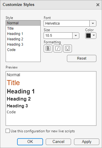
Customize Styles dialog box showing the selected Font, Size, Color, and Formatting for the Normal text style, and a preview of all the styles

Live Editor Controls: Add range sliders to live scripts

Add a range slider to your live script to select a range interactively. To add a range slider, go to the Live Editor tab, and in the Code section, select Control > Range Slider.

Range slider with the range [0 100] selected, assigned to the variable r

For more information, see Add Interactive Controls to a Live Script.

Live Editor Controls: Populate drop-down list items using additional variable types

You can now populate the items in a drop-down list using values stored in a categorical array, character array, cell array, or double array. Previously, only string arrays were supported.

You also can now edit the item labels after populating the items in a drop-down list using the values stored in a variable. Previously, the item labels were read-only.

For more information, see Link Variables to Controls.

Live Editor Controls: Restore default values for all controls

You can restore the default values for all controls in a live script. To restore the default values for all controls, right-click any control in the live script and select Restore Default Values for All Controls.

For more information, see Specify Default Values.

help Function: Get updated help text for functions, methods, and classes

The updated help text for functions, methods, and classes provides more consistent and uniform support across all products.

Use the help function to display abbreviated help text in the Command Window. For more extensive help, use the doc function instead.

Editor in MATLAB Online: View outline of your code using Outline panel

In the MATLAB Online Editor, you can use the Outline panel to view a high-level outline of scripts, functions, and classes. To view an outline of a file open in the Editor, go to the View tab, and in the Tools section, click Outline. To navigate to an area within your code file, double-click the related entry in the Outline panel.

For more information, see Edit and Format Code.

Outline panel showing the outline of the BankAccount class, which includes four properties and five methods

Editor TLC Support in MATLAB Online: View and edit TLC files with syntax highlighting and automatic indenting while typing

In MATLAB Online, the Editor displays Target Language Compiler (TLC) files with syntax highlighting for commands, comments, macros, and strings. In addition, the Editor automatically indents lines of code in TLC files while you type.

In MATLAB Online, you also can use preferences to configure how the Editor displays TLC files. On the Home tab, in the Environment section, click Preferences. Select MATLAB > Editor/Debugger > Other Languages > TLC, and adjust the options as needed.

Add-Ons in MATLAB Online: Update add-ons directly from Add-Ons panel

In MATLAB Online, you can update add-ons directly from the Add-Ons panel. To update an add-on, in the Installed section of the Add-Ons panel, click the Update button to the right of the add-on. The Add-Ons panel displays the Update button next to add-ons that have an update available.

To open the Add-Ons panel if it is not open, click the Add-Ons button in the sidebar on the left side of the MATLAB Online desktop. Alternatively, go to the Home tab, and in the Environment section, select Add-Ons > Add-Ons.

For more information, see Get and Manage Add-Ons.

Find Files in MATLAB Online: Manage list of search results and export as plain text

When searching using the Find Files panel in MATLAB Online, you can collapse or clear the list of search results. To collapse or clear the list of search results, click the Find Files actions button () at the top of the Find Files panel and select Collapse Results or Clear Results.

You also can export the list of search results as a plain text file (.txt) that can be viewed in an external text editor. To export the list, click the Find Files actions button () and select Export as Plain Text.

For more information, see Advanced Search in MATLAB Online.

New Desktop for MATLAB (Beta): Try new features including dark theme, an updated layout, and expanded search capabilities

The new desktop for MATLAB includes new and updated features, such as:

  • Dark theme support for the desktop, plots, and apps

  • An updated layout

  • Expanded search capabilities

  • A new figure window experience with a toolstrip, integrated side panels, and a new tabbed container

  • A new plain text file format for live scripts

  • A new Debugger panel and Source Control panel

  • Enhanced workflows for MATLAB projects

  • Improved screen reader support

  • Extension points

To try these new features, download the New Desktop for MATLAB (Beta) on File Exchange. For more information about these new features, see Get Started with the New Desktop for MATLAB (Beta).

Note

The new desktop for MATLAB is in beta development and should not be used for development or production activities. Report all feedback and issues directly to the development teams by using the Feedback button directly above the MATLAB Toolstrip.
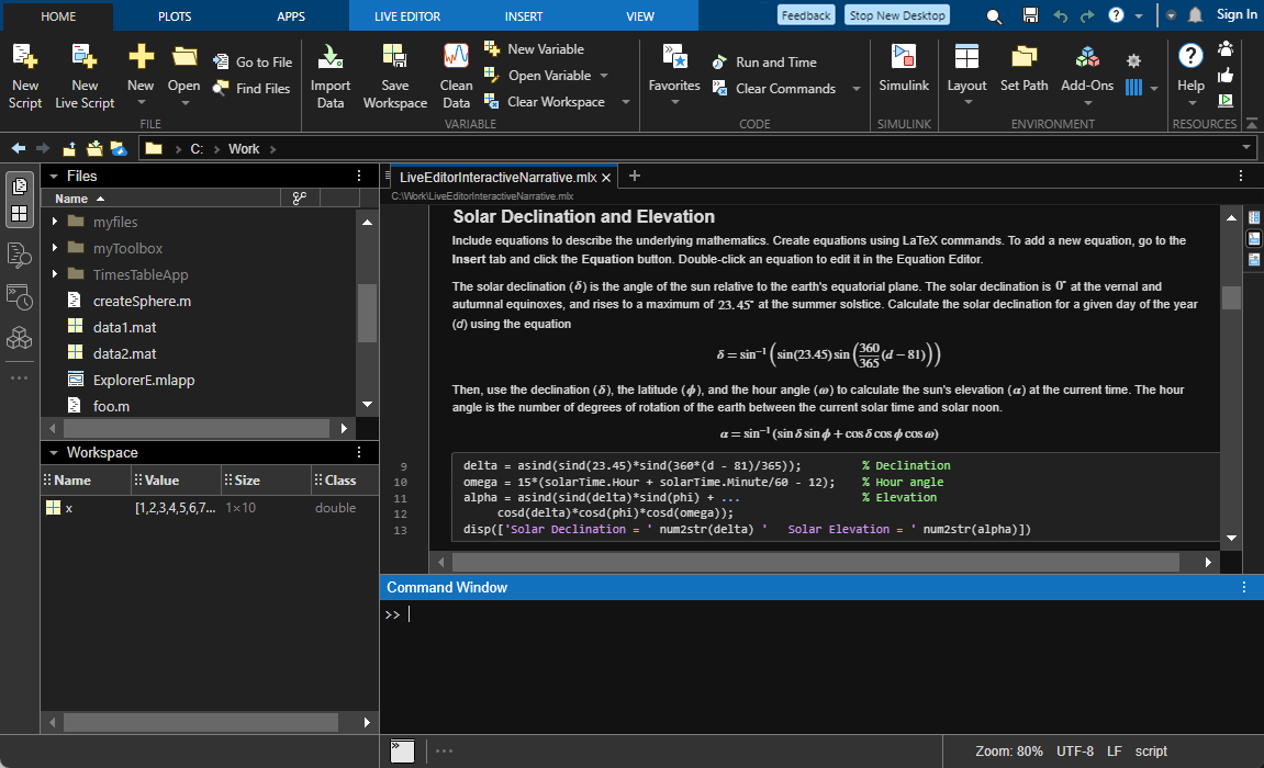
New desktop for MATLAB with all panels displayed with a dark background and light text

 Functionality being removed or changed

File version history in MATLAB Online is no longer supported

Behavior change

Restoring previous versions of a file in MATLAB Online is no longer supported. Previously, you could view the file version history and restore a previous version of a file by selecting it in the File Versions tab.

demo function no longer supports full product names

Behavior change

When you use the demo function to open examples for products other than MATLAB and Simulink, full product names are no longer supported. You must use the product short name instead.

For example, to open the examples for Computer Vision Toolbox™, use the command demo toolbox vision.

publish function will not longer support "entireFigureWindow" value for figureSnapMethod name-value argument

Still runs

For the publish function, specifying the figureSnapMethod name-value argument as "entireFigureWindow" will not be supported in a future release. Use the "entireGUIWindow", "print", or "getframe" values instead.

Language and Programming

 dbstop Function: Find missing semicolons by pausing execution on unsuppressed output

When debugging, you can use dbstop to pause execution when unsuppressed output is displayed because the line of code is not suppressed by a semicolon (;). Outputs that are displayed for other reasons, such as from disp or fprintf, do not stop execution.

Error Messages: Error text now indicates specific location in code

When possible, MATLAB adds caret symbols (^) in error messages beneath the code that led to the error. For example, calling the function getNumPermutations with a value of r greater than n causes an error in the second call to factorial. That second call is now specifically highlighted with carets in the error message.

function numPerms = getNumPermutations(n,r)
    numPerms = factorial(n)/factorial(n - r);
end
x = getNumPermutations(2,3)
Error using factorial (line 20)
N must be an array of real non-negative integers.

Error in getNumPermutations (line 2)
    numPerms = factorial(n)/factorial(n - r);
                            ^^^^^^^^^^^^^^^^

MATLAB also uses caret symbols to highlight inputs that fail argument validation in functions and class methods. For example, both the Height and Width input arguments for the function rectangleArea must be positive. The error message highlights which input does not pass validation.

function area = rectangleArea(Height,Width)
    arguments (Input)
        Height (1,1) {mustBePositive}
        Width (1,1) {mustBePositive}
    end
    area = Height*Width;
end
a = rectangleArea(5,4-7)
Error using rectangleArea (line 4)
 a = rectangleArea(5,4-7)
                     ^^^
Invalid argument at position 2. Value must be positive.

Debugging in MATLAB Online: View error breakpoint messages in Debugger panel

When the Pause on Errors or Pause on Warnings breakpoints are enabled and an error or warning occurs, the Debugger panel displays the resulting message and the location at which MATLAB is paused.
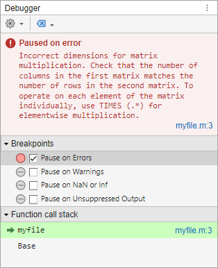
Debugger panel showing an incorrect dimension for matrix multiplication error with information about how to resolve the error, the file the error occurred in, and the code line

For more information about these error breakpoints, see Set Breakpoints.

matlab.lang.obfuscateNames Function: Obfuscate names of local variables, local functions, and nested functions

Use the matlab.lang.obfuscateNames function to obfuscate the names of local variables, local functions, and nested functions in MATLAB source code. While the commands pcode -R2022a and mcc -j provide obfuscation using P-code files, this matlab.lang.obfuscateNames function provides advanced obfuscation options.

MATLAB Vault: Access and identify existing MATLAB secrets in parallel environments

In parallel environments, you can access and identify existing secrets from your MATLAB vault using getSecret, getSecretMetadata, and isSecret. Creating, removing, and listing secrets in parallel environments is not supported.

Validation Functions: Validate arguments with matrix and vector shapes

Use the mustBeMatrix, mustBeRow, and mustBeColumn validation functions to enforce the dimensionality of an argument to be 2-D, a 1-by-N row vector, or an M-by-1 column vector, respectively. These functions extend the existing checks mustBeVector and mustBeScalarOrEmpty for robust size checking in argument and property validation.

For more information, see Function Argument Validation.

Handle Objects: Define weak references for handle objects

A weak reference to a handle object works much like a regular handle, but a weak reference does not prevent the object it references from being deleted. In other words, if an object is only referred to by weak references, MATLAB automatically deletes the object. Using weak references in applications like caches or data structures with back pointers can help simplify object cleanup.

You can use the WeakHandle property attribute to define a weak reference to the value of a property. You can also use the class matlab.lang.WeakReference to construct weak references to existing handle objects. For an overview and examples of the functionality, see Weak Reference Handles.

Object Serialization: Customize how objects are serialized and deserialized

Three new classes provide you with more control over customizing the serialization (saving) and deserialization (loading) processes:

Use these classes to preserve forward and backward compatibility for classes that you update over time. These classes add an extra level of control over serialization and deserialization beyond what the existing saveobj and loadobj methods provide. saveobj and loadobj will continue to work, but they cannot be combined with the new CustomElementSerialization mixin.

matlab.codeanalysis.validateConfiguration Function: View severity of issues in configuration file

The issues table returned by the matlab.codeanalysis.validateConfiguration function includes a column named Severity that shows the severity of an issue, specified as error, warning, or info.

The ErrorMessage and ErrorID columns have been renamed to Message and MessageID, respectively.

typecast Function: Convert data types using "like" syntax, and pass logical, character vector, and complex inputs

You can use the syntax typecast(X,"like",p) to convert the bit patterns of X to the same data type and complexity (real or complex) as the prototype p. You can also convert from and to logical or character vector data types, as well as complex numeric types. For more information, see typecast.

matlab.indexing.isScalarClass Function: Identify scalar classes

Use the matlab.indexing.isScalarClass function to identify scalar classes. The function returns true when its input is a function handle or an instance of a class that inherits from matlab.mixin.Scalar.

Class Diagram Viewer: Import classes from MATLAB packages

The Class Diagram Viewer app and the matlab.diagram.ClassViewer command-line API can import classes from MATLAB packages. For more information on packages, see Organize and Distribute Code Using MATLAB Package Manager.

 Functionality being removed or changed

mlintrpt function has been removed

Errors

The mlintrpt function has been removed. Use the Code Analyzer app instead to generate a report of code issues for a selected file or folder and its subfolders.

Class definition updates after path changes

Behavior change

When a new class definition is added to the path and it takes precedence over an old definition of the same name, MATLAB uses the new definition. MATLAB updates existing instances of the class the next time those instances are accessed. For more details, see Changing the Path to Update Class Definitions.

In previous releases, MATLAB immediately updated class definitions when the new definition was in a class folder (@-folder), but for classes defined in path folders, you had to clear the old definition before MATLAB recognized the new definition.

Default display for sparse matrices includes additional information

Behavior change

The default display for sparse matrices with double values now explicitly identifies the matrices as sparse. The display also now includes the dimensions, class, and number of nonzero entries in the matrix. For example:

A = [0 0 0 5; 0 2 0 0; 1 3 0 0; 0 0 4 0];
sparse(A)
ans =

  4×4 sparse double matrix (5 nonzeros)

   (3,1)        1
   (2,2)        2
   (3,2)        3
   (4,3)        4
   (1,4)        5

The default display for sparse matrices with logical values already identified the matrices as sparse and included the dimensions and class, but the display now also includes the number of nonzero entries.

Implicit default value for properties whose class is a subclass of matlab.mixin.Scalar

Behavior change

For properties whose class is a subclass of matlab.mixin.Scalar, MATLAB now creates an implicit default value by calling the no-argument constructor of the class. For example, if MyScalarClass is a subclass of matlab.mixin.Scalar, MATLAB calls the no-argument constructor of MyScalarClass to assign a default value to Prop1 in TestClass.

classdef TestClass
    properties
        Prop1 MyScalarClass
    end
end

Define an explicit default value for Prop1 if your class requires different behavior.

Implicit default value for properties whose class is an enumeration based on numeric or logical values

Warns

When MATLAB assigns a default value to a property whose class is an enumeration based on numeric or logical values, it currently uses the zero-based enumeration member if such a member exists. MATLAB chooses the zero-based member even if that member is not listed first in the enumeration definition. For example, in the class MyContainer, the default value of Prop1 is MyZero in R2024b.

classdef MyContainer
    properties
        Prop1 (1,1) MyEnum
    end
end
classdef MyEnum < uint8
    enumeration
        MyFirst (1)
        MyZero (0)
        MySecond (2)
        MyThird (3)
    end
end

In a future release, MATLAB will instead use the first listed enumeration member as the default, regardless of its underlying numeric value. In the case of MyContainer, the default value of Prop1 will be MyFirst. To avoid a warning in R2024b and a future change in behavior, assign MyEnum.MyZero as the default value for Prop1.

classdef MyContainer
    properties
        Prop1 (1,1) MyEnum = MyEnum.MyZero
    end
end

Defining classes: Using function syntax to define classes will not be supported in a future release

Still runs

Support for defining classes using function syntax will be removed in a future release. With appropriate code changes, replace existing function-based classes with classes defined using the classdef keyword.

Defining classes: Using schema.m will not be supported in a future release

Still runs

Support for classes defined using schema.m files will be removed in a future release. Replace existing schema-based classes with classes defined using the classdef keyword.

whos Function: Improved accuracy of array size information

Behavior change

The whos function returns a more accurate array size measurement in the Bytes column of the displayed list and in the bytes field of the output structure.

Data Analysis

 summary Function: Summarize array data and configure summary contents

The summary function can now display or return in a scalar structure a summary of array data, including numeric, logical, datetime, duration, and calendarDuration types. Previously, the function supported array data only when it was categorical.

You can configure the summary contents using one or more name-value arguments:

  • Statistics — Specify which statistics to compute.

  • Detail — For table or timetable data only, specify the level of table metadata detail to display in the summary.

  • DataVariables — For table or timetable data only, specify the variables to summarize.

 Compatibility Considerations

When you display a summary of a categorical array, the summary now always includes the number of undefined elements. Previously, the summary omitted the number of undefined elements if the array contained no missing values.

If you want to omit the number of undefined elements from the summary, specify the Statistics name-value argument. For example, summary(A,Statistics="counts") displays only the number of elements in each category.

isbetween Function: Specify numeric, nonnumeric, or tabular input data

Determine which elements are within a specified range using the isbetween function for any array, table, or timetable input data. Previously, supported only date and time input data.

For data in a table or timetable, you can return a table or timetable containing logical values instead of a logical array by using the OutputFormat name-value argument. You can also specify tabular variables to operate on by using the DataVariables name-value argument.

rmmissing and rmoutliers Functions: Define locations of missing entries or outliers using array or table

Define the locations of missing entries or outliers using a vector, matrix, table, or timetable. Specify the MissingLocations name-value argument of the rmmissing function or the OutlierLocations name-value argument of the rmoutliers function.

Previously, rmmissing did not support MissingLocations, and rmoutliers supported specifying OutlierLocations only as a vector or matrix.

Clean Outlier Data Live Editor Task and Data Cleaner App: Define outliers using range or workspace variable

In the Clean Outlier Data task and the Clean Outlier Data cleaning method in the Data Cleaner app, you can now detect outliers as elements outside of a range specified by an upper and lower threshold. Select the Range detection method.

In the Clean Outlier Data task, you can also define outliers using a logical workspace variable, where elements with a value of 1 (true) correspond to outliers. Select the Workspace variable detection method.

Experiment Manager: Improved interface for experiment setup and result analysis

In the Experiment Manager app, you can set up your experiment using an improved interface.

  • Create an initialization function that configures data or other experiment details before initiating the trial runs to reduce trial runtime. Previously, setup code was rerun for each trial.

  • Incorporate a suggested parameter for your experiment for some preconfigured experiment templates, such as the template that supports solving ordinary differential equations.

You can also efficiently analyze experiment results.

  • Your experiment function for a general purpose experiment can return an output containing multiple data types.

  • When an experiment runs using the sequential execution mode, you can stop or cancel the experiment. Clicking the Stop button finishes the current trial and ends experiment execution. Clicking the Cancel button immediately ends experiment execution.

  • When you select a trial in the results table, you can export the selected trial row to the MATLAB workspace as a table.

table and timetable Data Types: Specify the data types of table and timetable variables

The VariableTypes property of tables and timetables specifies the data types of their variables. For more information, see table and timetable.

timeseries2timetable Function: Convert events associated with timeseries objects to an event table associated with a timetable

You can convert timeseries objects that have events to a timetable that has an event table by using the timeseries2timetable function. When timeseries2timetable converts timeseries objects to a timetable, it also converts all associated tsdata.event event objects to an event table. Then the function attaches the event table to the timetable.

Before R2024b, timeseries2timetable ignored events when converting timeseries objects to a timetable.

Retime Timetable and Synchronize Timetables Live Editor Tasks: Specify custom function as local function or function handle

In the Retime Timetable and Synchronize Timetables Live Editor tasks, when you select the Custom function option for the General rule method, you can either select a locally defined function or specify a function handle.

To select a local function:

  1. Select Custom function.

  2. Select Local function from the next menu.

  3. If you want to add a new local function to the script, click New. The task generates template code for a custom aggregation function within the live script. To customize this code, edit it in the live script.

  4. Select the name of the local function from the select menu.

To specify a function handle:

  1. Select Custom function.

  2. Select Function handle from the next menu.

  3. Specify a function handle in the text box.

    You can specify a handle to a MATLAB function or write an anonymous function in the text box. For example, to specify mean as the function, type @mean in the text box.

Variables Editor in MATLAB Online: View variables with enhanced readability

Variables in the Variables editor in MATLAB Online have enhanced readability. The updated display has a streamlined look, including a simplified, borderless design and row striping for easier data review and analysis.

Variables editor view of a table with a borderless design and row striping

 Functionality being removed or changed

min and max functions no longer support specifying second input array as character array

Errors

The min and max functions now return an error if you specify the second input array as a character array. This change minimizes confusion with options that can be specified as character vectors, such as the missing value condition. To maintain the previous functionality, you can convert the second input array to double, for example, max(A,double(B),"includenan").

Data Import and Export

 Reading Online Data: Read remote data over HTTP and HTTPS using file operation, low-level I/O, datastore, video, and HDF5 functions

In addition to the existing support for reading remote data, you can now use the following functions to read data from primary online sources through an internet URL. Specify a filename that contains the protocol http:// or https://.

JSON: Read and write dictionaries in JSON files

You can read and write dictionaries in JSON files using the readdictionary and writedictionary functions.

Parquet: Import Parquet MAP data

You can read the Parquet MAP data type using parquetread. The function imports Parquet MAP data as cell arrays in which each cell is a table. Each table has two variables, Key and Value.

ZIP Files: Compress and extract password-protected files

Compress password-protected, encrypted ZIP files by specifying a password and encryption method with the zip function. Extract the contents of password-protected ZIP files by specifying a password with the unzip function.

Symbolic Links: Create and use symbolic links to manipulate files and folders

You can create and identify symbolic links using the createSymbolicLink and isSymbolicLink functions. Symbolic links allow you to refer to data in alternative locations.

You can delete, copy, and move files and folders using symbolic links. The deletion of a symbolic link has no effect on the target file, folder, or symbolic link. Use the ResolveSymbolicLinks name-value argument with the delete and rmdir functions, the CopyLinkBehavior name-value argument with the copyfile function, and the MoveLinkBehavior name-value argument with the movefile function.

Spreadsheet Files: Specify how to read merged cells from spreadsheets

You can specify how to read merged cells from spreadsheets using the MergedCellColumnRule and MergedCellRowRule name-value arguments with these functions:

For example, you can specify to place the data from merged cells in the leftmost or rightmost cell, duplicate data in all merged cells, omit rows or columns with merged data, or return an error.

Image Files: Automatically orient JPEG and TIFF images

If a JPEG or TIFF image file includes an Exif Orientation tag, you can automatically orient the image when reading it into MATLAB. Specify the AutoOrient name-value argument as true when you call the imread function.

The output structure of the imfinfo function includes AutoOrientedWidth and AutoOrientedHeight fields. These fields describe the width and height of the image data after the transformations specified by the Exif Orientation tag in the image file have been applied.

sonify Function: Convert numeric data to sound

The sonify function converts numeric data to sound using a frequency-based method and provides immediate playback capabilities. You can specify sonification parameters, such as frequency range, immediate playback control, and playback duration.

VideoReader Object: Read remotely stored video files

You can now read video files stored in remote locations, such as Amazon S3, Windows Azure® Blob Storage, and HDFS™, using the VideoReader object. The VideoReader object, however, does not support reading Motion JPEG 2000 (.mj2) files from a remote location.

FTP and SFTP: Specify time-out values for connections and transfers

You can specify the maximum amount of time allowed for a connection and for a transfer by using the ConnectionTimeout and TransferTimeout name-value arguments, respectively, with the ftp and sftp functions.

FTP: Enable TLS when connecting to FTP servers

When you connect to an FTP server using the ftp function, you can enable Transport Layer Security (TLS) using the TLSMode name-value argument.

SFTP: Connect to servers that require passphrases or certificates

You can connect to servers with passphrases and certificates by using the PrivateKeyPassphrase and CertificateFilename name-value arguments, respectively, with the sftp function.

HDF5 Interface: Use SZIP filter to read and write compressed datasets

You can write HDF5 datasets using SZIP compression. You can also read HDF5 datasets that have been compressed using SZIP compression.

In the high-level interface, use the SZIPEncodingMethod name-value argument of the h5create function to specify one of two methods for SZIP encoding. Optionally, if you specify SZIPEncodingMethod, you also can use the SZIPPixelsPerBlock name-value argument to specify the number of pixels (HDF5 data elements) per block.

In the low-level interface, use the H5P.set_szip function to specify SZIP compression when creating a new dataset.

These low-level functions accept the value "H5Z_FILTER_SZIP" for the filter input argument:

The H5Z.filter_avail function returns 1 (true) for the "H5Z_FILTER_SZIP" filter identifier.

HDF5 Interface: Work with file integrity checks (R2024b Update)

In the low-level HDF5 interface, you can enable and suppress file integrity checks using the H5P.set_relax_file_integrity_checks function. You can query the status of file integrity checks using the H5P.get_relax_file_integrity_checks function.

Starting in R2024b, file integrity checks are enabled by default. For compatibility considerations, see HDF5 file integrity checks are enabled by default (R2024b Update).

HDF Vgroup Interface: Define longer vgroup names and vgroup class names

In the HDF Vgroup (V) interface, you can define names of arbitrary length for vgroups and vgroup classes. For more information about the Vgroup interface, see hdfv.

Scientific File Format Libraries: HDF5 library upgraded to version 1.14.4.3 (R2024b Update)

The HDF5 library is upgraded to version 1.14.4.3.

 Functionality being removed or changed

Version 7.3 MAT files that contain variables of certain data types have decreased performance (R2024b Update)

Starting in R2024b, Version 7.3 MAT files use a newer version of the HDF5 library. This change causes decreased performance for some Version 7.3 MAT files that contain variables of any nonnumeric MATLAB data type besides char or logical. Functions that read from or write to MAT files, such as the load, save, and matfile functions, take up to twice as long to execute when called with Version 7.3 MAT files that contain variables of these data types.

HDF5 file integrity checks are enabled by default (R2024b Update)

Behavior change

Starting in R2024b, file integrity checks are enabled by default in the MATLAB HDF5 interface. When these checks are enabled, they fail for HDF5 datasets and attributes that contain a datatype that satisfies these two conditions:

  • The size of the datatype is at least 2 bytes.

  • The precision of the datatype is less than half of the size of the datatype.

As a result, the behavior of these high-level HDF5 functions has changed:

  • The h5read, h5readatt, and h5writeatt functions now issue errors for datasets and attributes that fail file integrity checks. Previously, these functions did not issue errors for such datasets or attributes. To read data or read or write attributes in such situations, use the H5P.set_relax_file_integrity_checks function and the low-level HDF5 interface.

  • The h5disp and h5info functions now issue warnings for datasets and attributes that fail file integrity checks. These functions omit information about such datasets and attributes from their outputs. Previously, these functions did not issue warnings in this situation and included information about those datasets and attributes in their outputs. The warnings take this form:

    Warning: Unable to read 'datasetName' from the file. A portion of the file may be corrupt.
    
    You can suppress file integrity checks in the low-level HDF5 interface using the H5P.set_relax_file_integrity_checks function, but not in the high-level HDF5 interface. This table shows how to update your code to use the low-level HDF5 interface.

R2024a and EarlierStarting in R2024b
myData = h5read("myFilename.h5","myDatasetName");
fapl = H5P.create("H5P_FILE_ACCESS");
H5P.set_relax_file_integrity_checks(fapl,"H5F_RFIC_UNUSUAL_NUM_UNUSED_NUMERIC_BITS")
fid = H5F.open("myFilename.h5","H5F_ACC_RDONLY",fapl);
dset_id = H5D.open(fid,"myDatasetName");
myData = H5D.read(dset_id);
H5D.close(dset_id)
H5F.close(fid)
H5P.close(fapl)
myAttrValue = h5readatt("myFilename.h5","myDatasetName","myAttrName");
fapl = H5P.create("H5P_FILE_ACCESS");
H5P.set_relax_file_integrity_checks(fapl,"H5F_RFIC_UNUSUAL_NUM_UNUSED_NUMERIC_BITS")
fid = H5F.open("myFilename.h5","H5F_ACC_RDONLY",fapl);
dset_id = H5D.open(fid,"myDatasetName");
attrID = H5A.open(dset_id,"myAttrName");
myAttrValue = H5A.read(attrID);
H5A.close(attrID)
H5D.close(dset_id)
H5F.close(fid)
H5P.close(fapl)
h5writeatt("myFilename.h5","myDatasetName","myAttrName",myAttrValue);
fapl = H5P.create("H5P_FILE_ACCESS");
H5P.set_relax_file_integrity_checks(fapl,"H5F_RFIC_UNUSUAL_NUM_UNUSED_NUMERIC_BITS")
fid = H5F.open("myFilename.h5","H5F_ACC_RDWR",fapl);
dset_id = H5D.open(fid,"myDatasetName");

% Assumes myAttrName is an existing attribute.
% If it does not already exist, use H5A.create.
attrID = H5A.open(dset_id,"myAttrName");

H5A.write(attrID,"H5ML_DEFAULT",myAttrValue)
H5A.close(attrID)
H5D.close(dset_id)
H5F.close(fid)
H5P.close(fapl)

Mathematics

 Solve ODE Live Editor Task: Interactively solve systems of ordinary differential equations

Use the Solve ODE task in the Live Editor to interactively solve a system of ordinary differential equations. You can specify the ODE structure and advanced problem details, select the solver, and visualize the solution in a plot. To add the task to a live script in the Live Editor, click Task on the Live Editor tab and select Solve ODE.

ode Object: Specify ODE as implicit

You can now specify the Solver property for ode objects as "ode15i" for implicit ODEs. Alternatively, you can specify whether your ODE is implicit by setting the new EquationType property for ode objects to "standard" (default) or "fullyimplicit". If you specify the Jacobian when the equation type is "fullyimplicit", the Jacobian must be a function handle or cell array.

For example, F = ode(ODEFcn=@myFcn,EquationType="fullyimplicit",Jacobian=@Fjac) specifies an implicit ODE.

ode Object: Detect stiffness to change solver after creating ode object

You can change the solver after creating an ode object by using the selectSolver method. Use the DetectStiffness name-value argument to incorporate a stiffness detection heuristic when selecting a solver.

For example, d.Solver = selectSolver(d,DetectStiffness="on") changes the solver for ode object d by using a stiffness detection heuristic.

ode Options: Set minimum step size for several ODE solvers

You can set a lower bound on the size of any step taken by MATLAB ODE solvers by specifying the MinStep name-value argument of the odeset function.

See the SolverOptions property of the ode object for a list of the solvers that support setting a minimum step size.

lsqminnorm Function: Apply Tikhonov regularization to least-squares solution

You can apply Tikhonov regularization to the least-squares solution of the lsqminnorm function by specifying the RegularizationFactor name-value argument as a real number. Specify the regularization factor lambda to return a solution X that minimizes norm(A*X-B)^2 + lambda^2*norm(X)^2 for each column of X.

For example, X = lsqminnorm(A,B,RegularizationFactor=1e-6) specifies a Tikhonov regularization factor of 1e-6.

isapprox Function: Determine approximate equality of elements in two arrays

Determine approximate equality of elements in two arrays and return a logical array using the isapprox function. You can define the maximum difference between approximately equal elements by specifying a tolerance level or the relative and absolute tolerances.

layoutcoords Function: Calculate node and edge coordinates for the layout of a graph or digraph

Use the layoutcoords function to calculate the node and edge coordinates used when plotting a graph or digraph object. While the layout function changes the layout of an existing GraphPlot object, layoutcoords enables you to obtain the coordinates that would be used by a layout method without plotting the network.

polyshape Object: Control whether subtract and xor methods simplify output

You can control whether the subtract and xor methods of polyshape simplify their output by specifying the Simplify name-value argument, which can be either true (default) or false. By default, the methods return a well-defined polygon by resolving boundary intersections and improper nesting and by removing duplicate points and degeneracies. However, you can specify Simplify=false to gain performance when performing a series of subtractions or exclusive-or operations. In this case, you can simplify the output once at the end either by specifying Simplify=true in the final method call or by using the simplify method on the final output polygon.

MATLAB Support Package for Quantum Computing: Solve QUBO problems using QAOA (November 2024, Version 24.2.2)

You can solve a Quadratic Unconstrained Binary Optimization (QUBO) problem using the quantum approximate optimization algorithm (QAOA). Specify the algorithm for the solve function as a qaoa object. The resulting solution is a quboResult object that contains a qaoaResult object.

You can also solve a max-cut problem using the solve function. Convert the max-cut graph to an equivalent QUBO formulation by using the maxcut2qubo function, which returns a qubo object. For more information, see Solve Max-Cut Problem Using QAOA.

MATLAB Support Package for Quantum Computing: Calculate expected value and convert QUBO to Ising (February 2025, Version 24.2.4)

You can calculate the expected value of a quantum circuit or state using the observe function. Specify the basis to calculate the expected value in by using an observable object or Hermitian matrix.

You can also convert a QUBO problem to an equivalent Ising observable using the qubo2ising function, which returns an observable object.

 Functionality being removed or changed

ind2sub function no longer supports scalar input for array size

Errors

When you use the ind2sub function, the input argument for the size of the array must be a vector of positive integers with two or more elements. In previous releases, ind2sub(sz,ind) treated a scalar input size sz as the number of rows in the array and assumed the size of the other dimensions to be 1. For example:

[row,col] = ind2sub(6,[2 3 4])
row =

     2     3     4


col =

     1     1     1
Starting in R2024b, a scalar input for sz results in an error. Instead, you must specify sz as a vector of positive integers with two or more elements. For example:
[row,col] = ind2sub([6 1],[2 3 4])

MATLAB Support Package for Quantum Computing: run function no longer supports OptimizationLevel argument (January 2025, Version 24.2.3)

Errors

The run function no longer supports the OptimizationLevel name-value argument. Code that uses this argument generates an error. This change affects all versions of MATLAB Support Package for Quantum Computing.

Graphics

 violinplot Function: Visualize grouped numeric data by using violin plots

To create violin plots for grouped numeric data, use the violinplot function. Each violin plot displays the kernel density estimate for a group in the input data. If you specify a matrix of input data, violinplot creates a separate violin plot for each column in the matrix. You can also specify a positional grouping variable to split your data into groups.

Violin plot that shows distributions of diastolic blood pressure for smokers and nonsmokers

 compassplot Function: Create one or more compass plots in polar axes

Use the compassplot function to plot one or more sets of arrows originating from the origin in polar coordinates. This function is recommended over the compass function because this function uses a PolarAxes object, which provides more options for customization. For example, you can set PolarAxes properties to display either degree or radian theta units, adjust theta- and r-axis limits, or adjust aspects of the tick labels.
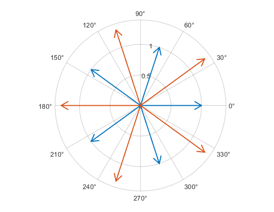
Compass plot with five blue arrows and five red arrows emanating from the origin

constantplane Function: Create infinite planes

Use the constantplane function to create infinite planes for highlighting regions of interest in 3-D plots. This function creates semitransparent gray planes by default, but you can change the color and transparency by setting properties.
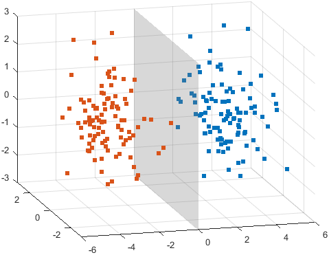
Two 3-D distributions of scattered points with a semitransparent gray plane between them

Legends: Control width of icons

Control the width of the legend icons and the width of the legend box by setting the IconColumnWidth property of a Legend object.

If the legend contains only marker icons, MATLAB automatically minimizes the white space around the icons. Previously, legends included extra white space around the marker icons.

For example, these three legends are the same except for their IconColumnWidth values (30, 40, and 10, respectively).
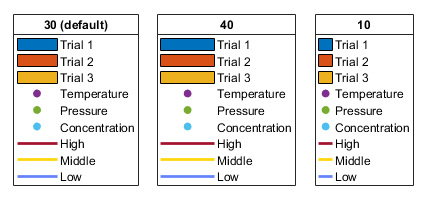
Three legends that have different IconColumnWidth values. As the IconColumnWidth value decreases, certain icons become narrower, and the legend box becomes narrower.

Pie Charts and Donut Charts: Control slice order and number of slices

Simplify pie charts and donut charts with large numbers of slices by setting properties that control the order and number of slices. Use the DisplayOrder property to arrange slices by size, and use the NumDisplayWedges property to specify the number of slices to display separately (the remaining slice data is grouped together as a slice labeled "Others").

Other useful properties include:

  • ShowOthers — Show or hide a slice labeled "Others" to represent values not shown as individual slices. For example, <undefined> categorical values are represented in the "Others" slice.

  • WedgeDisplayNames — Return the labels of the slices shown in the chart.

  • WedgeDisplayData — Return the data values of the slices shown in the chart.

For example, these two donut charts represent the same data, but the chart on the right has a NumDisplayWedges property value of 3 and a ShowOthers property value of "on".
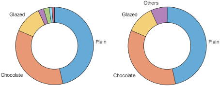
Two donut charts containing three common slices, which are labeled "Plain", "Chocolate", and "Glazed". One of the charts has four unlabeled narrow slices. The other chart combines the data from the four narrow slices into one slice labeled "Others".

Bar Charts: Add labels to ends of bars

Add labels to the ends of bars and position them using the Labels and LabelLocation properties of a Bar object. You can also adjust aspects of the font by setting the LabelColor, FontName, FontSize, FontWeight, and FontAngle properties. To create the labels with LaTeX markup, set the Interpreter property.
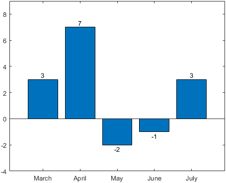
Bar chart with positive and negative bars. The bar labels are above the positive bars and below the negative bars.

ConstantLine Object: Control text label color

Use the LabelColor property to control the color of the text label of a ConstantLine object created with the xline or yline function.
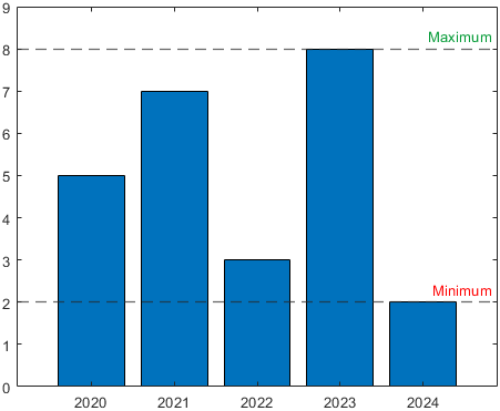
Bar chart with two horizontal dashed lines that span the width of the chart. One line is at the height of the tallest bar with a green label "Maximum". The other line is at the height of the shortest bar with a red label "Minimum".

tiledlayout Function: Create layouts without specifying dimensions or tile arrangement

Call the tiledlayout function without specifying the dimensions (m and n) or the tile arrangement argument. When you omit these arguments, tiledlayout creates a layout in the "flow" configuration, which can accommodate any number of tiles.

savefig Function: Specify MAT file version

Specify the MAT file version as "-v7.3", "-v7", or "-v6" when you create FIG files using the savefig function.

The "-v7.3" option supports FIG-files that are larger than 2 GB, and the "-v7" option supports up to 2 GB files. The "-v6" option stores the file using the MATLAB Version 5 format.

Name-Value Arguments: Set properties when you call pcolor, sphere, cylinder, and other plotting functions

Specify name-value arguments to set properties when you call pcolor, sphere, cylinder, streamline, waterfall, ellipsoid, feather, surfl, or ribbon. Previously, these functions did not support name-value arguments.

For example, specify the FaceColor and EdgeColor name-value arguments when you call pcolor.

pcolor(peaks,FaceColor="interp",EdgeColor="none")

Graphics in MATLAB Online: Copy images to clipboard

Now you can use the copygraphics function to copy images to the clipboard in MATLAB Online. Previously, you could use the copygraphics function only in an installed version of MATLAB.

 Functionality being removed or changed

piechart and donutchart show undefined categorical values by default

Behavior change

The piechart and donutchart functions now include undefined categorical values and show them in a slice labeled "Others" by default. Previously, the functions excluded undefined values from the calculation of the Proportions property, and the resulting chart did not include undefined values. This change makes it easier to understand the nature of categorical data in the chart.

For example, create a pie chart using a categorical array containing three undefined values (""). In R2024a, the chart excludes the undefined values. In R2024b, the chart contains a slice labeled "Others" to represent the undefined values.

cats = categorical(["Peach" "Apple" "Apple" "Apple" ...
                    "Pecan" "Pecan" "Pumpkin" "" "" ""]);
piechart(cats,LabelStyle="name")
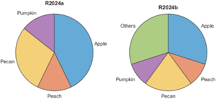
Two pie charts created using the same categorical data including three undefined values in R2024a and R2024b. The chart created in R2024b contains a slice labeled "Others", which corresponds to the three undefined values. The chart created in R2024a does not have a slice labeled "Others".

To exclude the "Others" slice from the chart and exclude the undefined values from the Proportions calculation, set the ShowOthers property to "off".

piechart(cats,LabelStyle="name",ShowOthers="off")

savefig function saves FIG files that are no longer compatible with R2014a and earlier releases

Behavior change

The savefig function now saves FIG files using the compact format by default. As a result, if you save FIG files in R2024b, you can open them only in R2014b and later releases. Previously, savefig stored an extra copy of the figure that you could open in R2014a and earlier releases. This change reduces the file size by approximately 50%.

If you specify the "compact" option when you call savefig, MATLAB stores the same compact version of the FIG file that it saves by default. Thus, the "compact" option is unnecessary, but it still runs in R2024b without error. In a future release, the "compact" option will be removed.

x-axis limits of stem plots are padded by default

Behavior change

Plots created with the stem function now have padding on the right and left sides of the x-axis to prevent overlap with the edges of the plot box.
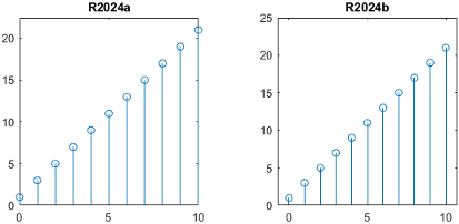
Two stem plots of the same data. One plot was created in R2024a and the stems at x=0 and x=10 overlap with the edges of the plot box. The other plot, created in R2024b, has a margin of padding between the plot box and the stems. Thus, all of the stems in the R2024b plot are clearly visible.

To preserve the appearance from previous releases, use the xlim function to adjust the limits of the x-axis. For example, if the range of the x-coordinates is [0,10], set the x-axis limits to [0,10].

x = 0:10;
y = (2*x) + 1;
stem(x,y)
xlim(gca,[0 10])

Passing multidimensional arrays to isgraphics and ishghandle returns output of same size

Behavior change

Passing arrays that have three or more dimensions to the isgraphics and ishghandle functions returns arrays of the same size as the input. Previously, isgraphics and ishghandle returned 2-D arrays when the input had three or more dimensions. The higher dimensions were collapsed into the second dimension. For example, if the input was a 2-by-4-by-5 array, the output was a 2-by-20 array.

If you pass a scalar, 1-D, or 2-D array to either function, the output is the same size as in previous releases.

If you use nested calls to the all or any function, update your code to use the "all" argument instead of the nested function calls to preserve the shape of the output.

For example, this code returns a scalar logical value in R2024a. In R2024b, it returns a 1-by-1-by-4 array of logical values.

h = gobjects(2,3,4);
all(all(isgraphics(h)))

To preserve the scalar output, call the all function once with the "all" argument. The result is a scalar logical value.

h = gobjects(2,3,4);
all(isgraphics(h),"all")

hgsave and support for saving legacy FIG files will be removed

Still runs

The hgsave function will be removed in a future release. Use savefig to save FIG files instead. The savefig function supports the same arguments and syntaxes that the hgsave function supports, and it saves FIG files that are compatible with R2014b and later releases.

When hgsave is removed, you will no longer be able to save FIG-files compatible with R2014a and earlier releases.

hold all is not recommended

Still runs

The "all" option of the hold function is not recommended. Specify the "on" option instead, which has the same effect. However, there are no plans to remove the "all" option.

Not RecommendedRecommended

hold all

hold on

hold("all")

hold("on")

hold(ax,"all")

hold(ax,"on")

compass is not recommended

Still runs

The compass function is not recommended. Use the compassplot function instead. The compassplot function uses a PolarAxes object, which provides more options for customization. For example, you can set PolarAxes properties to display either degree or radian theta units, adjust theta- and r-axis limits, or adjust aspects of the tick labels. However, there are no plans to remove the compass function.

Like other polar plotting functions, compassplot accepts polar coordinates instead of Cartesian coordinates. Use the cart2pol function to convert your data. This table shows some typical usages and how to update your code to use compassplot.

ScenarioNot RecommendedRecommended

Plot vectors of coordinates — Convert the Cartesian values of u and v to polar coordinates before passing them to compassplot.

compass(u,v) 

[theta,rho] = cart2pol(u,v);
compassplot(theta,rho)

Plot matrices of coordinates — The compass function plots all of the arrows using the same color. compassplot uses a different color for each matrix column. To make all the arrows the same color, set the SeriesIndex name-value argument to 1.

compass(u,v)

[theta,rho] = cart2pol(u,v);
compassplot(theta,rho,SeriesIndex=1)

Plot complex values

compass(Z)

compassplot(Z)

Specify line style and color

compass(u,v,"--r")

[theta,rho] = cart2pol(u,v);
compassplot(theta,rho,LineStyle="--",Color="r")

Calling legend with multiple outputs will not be supported

Warns

Calling the legend function with multiple output arguments returns a warning that the syntax will be removed in a future release.

[lgd,icons,plots,txt] = legend(...)

This syntax creates a legend that does not support some functionality. For example, you cannot add a title to the legend or specify the number of legend columns. Also, the legend does not automatically update when you add or remove data series from the axes.

Instead, return the Legend object and set its properties. For a complete list, see Legend Properties.

lgd = legend(...)

opengl function will be removed

Warns

The opengl function returns a warning that it will be removed in a future release. This function enables you to query or change the renderer that MATLAB uses.

  • To query the renderer, use the rendererinfo function instead of the opengl function.

  • Changing the renderer will no longer be necessary when the function is removed.

axis function no longer returns limit selection mode, visibility, and y-axis direction

Errors

Calling this three-output syntax of the axis function is no longer supported.

[m,v,d] = axis('state')

You can get the same information by querying these Axes properties:

App Building

uibutton and uitogglebutton Functions: Specify HTML markup and display equations in button text

Enable text markup for buttons created using the uibutton and uitogglebutton functions by setting the Interpreter property. Specify the interpreter as "html", "latex", "tex", or "none".

For more information, see Button, StateButton, or ToggleButton.

App Designer: Add UI components that span multiple grid cells more easily

In Design View, you can interactively add UI components that span multiple cells in a grid layout manager by dragging the component over multiple cells before dropping it on the canvas.

For more information, see Use Grid Layout Managers in App Designer.
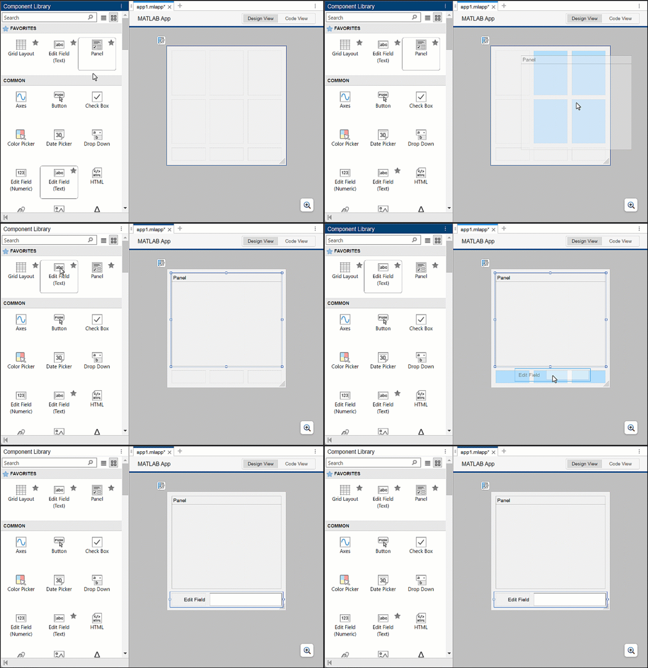
Animation of adding a panel and an edit field, each spanning multiple grid cells, to a grid layout manager in App Designer

App Designer: View errors directly in Code View when debugging an app

When you debug an app in App Designer with the Pause on Errors option selected, Code View displays any error that occurs next to the line of code that caused it. Previously, the error was displayed only in the MATLAB Command Window.

App Designer: Convert between text edit fields and numeric edit fields

To convert one type of edit field to another, right-click the edit field on the canvas and select Replace With. Then, select the edit field type to convert to. Replacing one edit field with another preserves relevant property values, such as font properties and callbacks that exist for both components.

App Testing Framework: Programmatically interact with alert and confirmation dialog boxes

You can programmatically interact with a modal dialog box in front of a figure window by using two new methods in the app testing framework:

  • To select an option in a confirmation dialog box, use the chooseDialog method.

  • To dismiss an alert or confirmation dialog box, use the dismissDialog method.

App Testing Framework: Specify location of gesture on figures that use nonpixel units

You can specify the location of a gesture on a UI figure that uses any unit of measurement. In previous releases, the press, drag, hover, and chooseContextMenu methods let you specify coordinates only for figures whose Units property is set to "pixels".

For example, create a figure with its Units property set to "normalized". Then, programmatically press a point near the lower-left corner of the figure.

fig = uifigure(Units="normalized");

testCase = matlab.uitest.TestCase.forInteractiveUse;
testCase.press(fig,[0.1 0.1])

 Functionality being removed or changed

Figure menu bar and toolbar are unaffected by reset

Behavior change

When you reset the properties of a Figure object, for example by using reset or clf("reset"), the MenuBar and ToolBar properties are unaffected. For more information, see reset and clf.

dismissAlertDialog method is not recommended

Still runs

The dismissAlertDialog method is not recommended. Use dismissDialog instead. There are no plans to remove dismissAlertDialog. However, the dismissDialog method provides more functionality and is not limited to alert dialog boxes. For example, you can use the dismissDialog method to close an alert dialog box or a confirmation dialog box.

This table shows how to update your code to use dismissDialog instead.

Not RecommendedRecommended
fig = uifigure;
uialert(fig,"File not found","Invalid File")

testCase = matlab.uitest.TestCase.forInteractiveUse;
testCase.dismissAlertDialog(fig)
fig = uifigure;
uialert(fig,"File not found","Invalid File")

testCase = matlab.uitest.TestCase.forInteractiveUse;
testCase.dismissDialog("uialert",fig)

Specifying location of gesture on axes or UI axes with active right y-axis is no longer supported

Errors

Using the press, drag, hover, or chooseContextMenu method to specify the location of a gesture on axes or UI axes with an active right y-axis is no longer supported. In previous releases, when you specify the location on axes or UI axes with an active right side, the app testing framework interprets that location with respect to the left y-axis, which can cause the gesture to occur at an unexpected location or fail.

If your chart has two y-axes, activate the left side before performing a gesture at a specified location on the axes or UI axes. This table shows an example of how you can update your code.

BeforeAfter
fig = uifigure; 
ax = axes(fig); 
yyaxis(ax,"left")
plot(ax,1:10)
yyaxis(ax,"right") 
plot(ax,10:-1:1)

testCase = matlab.uitest.TestCase.forInteractiveUse;
testCase.press(ax,[5 5])
fig = uifigure; 
ax = axes(fig); 
yyaxis(ax,"left")
plot(ax,1:10)
yyaxis(ax,"right") 
plot(ax,10:-1:1)

testCase = matlab.uitest.TestCase.forInteractiveUse;
yyaxis(ax,"left")
testCase.press(ax,[5 5])

Performance

datetime Format Parsing: Improved performance when parsing common formats that include localized names or time zone offsets

datetime format parsing performance is significantly faster when parsing common formats that include localized names or time zone offsets. This list shows a few examples of such formats, which are part of ongoing efforts to improve datetime format parsing performance:

  • dd-MMM-uuuu HH:mm:ss

  • MMMM/dd/uuuu

  • QQQ-uuuu

  • uuuu-MM-dd HH:mm:ss Z

  • uuuu-MM-dd HH:mm:ss.SSS xxx

For example, this code creates a string array of dates that use a localized abbreviation for the month of April. The dates in the string array use the dd-MMM-uuuu HH:mm:ss format, where the MMM specifier represents the abbreviated month name. Then the code uses the datetime function to parse and convert the string array. The code is about 17x faster than in the previous release.

function timingTest
s = "23-Apr-2024 11:30:" + randi([10,59],10000,1);
for i = 1:100
    d = datetime(s, ...
        InputFormat="dd-MMM-uuuu HH:mm:ss", ...
        Locale="en_US");
end
end

The approximate execution times are:

R2024a: 4.75 s

R2024b: 0.27 s

Similarly, this code creates a string array of dates that have a time zone offset of -0400. The dates in the string array use the uuuu-MM-dd HH:mm:ss.SSS Z format, where the Z specifier represents the time zone offset. Then the code uses the datetime function to parse and convert the string array. The code is about 5.8x faster than in the previous release.

function timingTest
s = "2024-04-23 11:32:48." + randi(999,10000,1) + " -0400";
for i = 1:100
    d = datetime(s, ...
        InputFormat="uuuu-MM-dd HH:mm:ss.SSS Z", ...
        TimeZone="local");
end
end

The approximate execution times are:

R2024a: 6.35 s

R2024b: 1.10 s

In both cases, the code was timed on a Windows 11, AMD EPYC 74F3 24-Core Processor @ 3.19 GHz test system using the timeit function.

timeit(@timingTest)

median Function: Improved performance when computing weighted median

The median function shows improved performance when you specify a weighting scheme. For example, this code computes the weighted median of a 600-by-10 matrix. The code is about 1.8x faster than in the previous release.

function timingTest
A = rand(600,10);
W = rand(600,1);

for i = 1:3e3
   median(A,Weights=W);
end
end

The approximate execution times are:

R2024a: 1.00 s

R2024b: 0.55 s

The code was timed on a Windows 11, AMD EPYC 74F3 24-Core Processor @ 3.19 GHz test system using the timeit function.

timeit(@timingTest)

fillmissing Function: Improved performance when filling numeric entries using nearest neighbor rows

The fillmissing function shows improved performance when you specify the fill method as "knn" for numeric data and use the Euclidean or scaled Euclidean distance function to find the nearest neighbor rows. The improvement is most significant when the length of the input data along the operating dimension is small.

For example, this code fills the NaN values in an 800-by-10 matrix using the nearest neighbor rows. The code is about 2.8x faster than in the previous release.

function timingTest
A = rand(800,10);
A(A>0.95) = NaN;

for i = 1:2e2
   F = fillmissing(A,"knn");
end
end

The approximate execution times are:

R2024a: 1.00 s

R2024b: 0.36 s

The code was timed on a Windows 11, AMD EPYC 74F3 24-Core Processor @ 3.19 GHz test system using the timeit function.

timeit(@timingTest)

isprime Function: Improved performance when determining which array elements are prime

The isprime function shows improved performance when determining whether the integer elements of an array are prime. For example, this code checks if the elements of a 1-by-1,000,000 vector of integers are prime. The code is about 20x faster than in the previous release.

function timingTest
x = 1:1e6;
tf = isprime(x);
end

The approximate execution times are:

R2024a: 2.81 s

R2024b: 0.14 s

The code was timed on a Windows 11, AMD EPYC 74F3 24-Core Processor @ 3.19 GHz test system using the timeit function.

timeit(@timingTest)

simplify Function: Improved performance when simplifying polyshape objects with many boundaries

The simplify function shows improved performance when operating on polyshape objects with many boundaries. For example, this code simplifies a polyshape object with 11,100 vertices. The code is about 23x faster than in the previous release.

function t = timingTest
n = 300;
x = (1:n)'*[sind(0:10:360),NaN];
y = (1:n)'*[cosd(0:10:360),NaN];
p = polyshape(x(:),y(:),Simplify=false);

f = @() simplify(p);

t = timeit(f);
end

The approximate execution times are:

R2024a: 0.28 s

R2024b: 0.012 s

The code was timed on a Windows 11, AMD EPYC 74F3 24-Core Processor @ 3.19 GHz test system by calling the timingTest function.

waitbar Function: Improved performance when updating wait bar dialog box in loop

Updating a wait bar dialog box created using the waitbar function shows improved performance when the updates happen many times in a loop. For example, this code updates a wait bar dialog box progress bar and message while approximating the value of π. The code is about 3.9x faster than in the previous release.

function timingTest
f = waitbar(0,"1",Name="Approximating pi...");
pisqover8 = 1;
denom = 3;
valueofpi = sqrt(8*pisqover8);
steps = 20000;

tic
for step = 1:steps
    waitbar(step/steps,f,sprintf('%12.9f',valueofpi))
    pisqover8 = pisqover8 + 1/(denom*denom);
    denom = denom + 2;
    valueofpi = sqrt(8*pisqover8);
end
toc

delete(f)
end

The approximate execution times are:

R2024a: 58.7 s

R2024b: 14.9 s

The code was timed on a Windows 11, AMD EPYC 74F3 24-Core Processor @ 3.19 GHz test system by calling the timingTest function.

Plot Animations: Improved performance when updating charts that have legends in loop

Updating graphics properties in a loop shows improved performance when the axes object contains multiple graphics objects and a legend. The improvement increases with the number of graphics objects in the axes.

For example, plot 10 lines and add a legend.

axes
hold on
numLines = 10;
for i = 1:numLines
    plot(i:i+10);
end
legend(Location="eastoutside")

Calculate values of a sine wave and store them as y. Create another line, p1, with NaN coordinate values. Animate the line in a loop by appending y(i) to the YData property of p1 at each iteration. This code is about 5x faster than in the previous release.

% Calculate sine values and create p1
x = 1:0.05:11;
y = sin(x)*10+10;
p1 = plot(x,nan(1,numel(x)));

% Animate p1
tic
for i = 1:numel(x)
    p1.YData(i) = y(i);
    drawnow
end
toc

The approximate execution times are:

R2024a: 14.14 s

R2024b: 2.89 s

The code was timed on a Windows 11, Intel Xeon CPU W-2133 @ 3.60 GHz test system.

Plots in Apps: Improved performance when creating surface plots of large data sets

In apps, creating surface plots of large data sets shows improved performance. For example, create an app window using the uifigure function, and create an axes object using the axes function. Call the drawnow function to complete the figure and axes setup. Then plot a 1000-by-1000 sampling of the peaks data set using the surf function. The code is about 1.3x faster than in the previous release.

% Create app window and axes
f = uifigure;
a = axes(f);
drawnow

% Plot surface
tic
surf(a,peaks(1000), ...
    FaceColor="interp",EdgeColor="none")
drawnow
toc

The approximate execution times are:

R2024a: 0.478 s

R2024b: 0.356 s

The code was timed on a Windows 11, AMD EPYC 74F3 24-Core Processor @ 3.19 GHz test system that has an NVIDIA A16-2Q GPU with 2 GB RAM.

Create Plot Live Editor Task: Improved loading performance

Loading the Create Plot task in the Live Editor is faster in R2024b than in R2024a. When you add the task to a live script, it takes less time for the task to appear in the Live Editor.

For example, if you add the Create Plot task to a new script in the Live Editor, the task appears about 1.2x faster than in the previous release.

The approximate load times are:

R2024a: 19.9 s

R2024b: 16.4 s

If you add another Create Plot task to the same live script, the additional task appears about 1.4x faster than in the previous release.

The approximate load times are:

R2024a: 5.7 s

R2024b: 4.0 s

The actions were timed on a Windows 11, Intel Xeon Gold 6246R CPU @ 3.40 GHz test system.

Software Development Tools

Project API: Specify dependency analysis scope

When you analyze a project using the updateDependencies function, you can specify the dependency analysis scope. For example, to analyze dependencies inside add-ons, use updateDependencies(currentProject,AnalyzeAddOns=true).

Project API: Label multiple project files at once

You can programmatically attach a label to multiple project files at once using addLabel. You can also detach a label from multiple files using removeLabel.

Dependency Analyzer: Find required packages and missing package dependencies

When you run a dependency analysis on your code, the Dependency Analyzer lists the required packages in the Add-Ons section of the Properties pane. For more information, see Find Required Products and Add-Ons.

The Dependency Analyzer also flags any missing package dependencies in the Problems section. For more information, see Investigate and Resolve Problems.
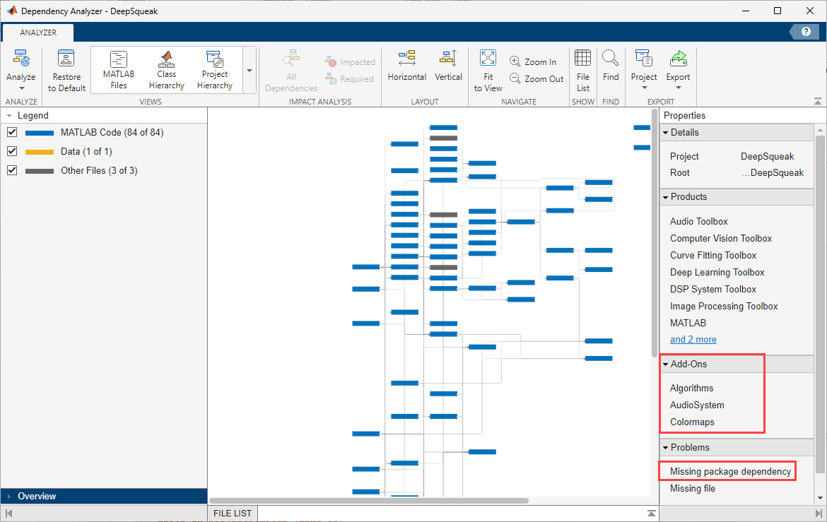
Dependency Analyzer with a toolstrip at the top, Legend pane on the left, Properties pane on the right, and the dependency graph in the middle. The Properties pane includes Details, Products, Add-Ons, and Problems sections.

Source Control in MATLAB Online: Expanded support for Git workflows

MATLAB Online now provides expanded support for Git workflows.

  • Annotate lines in the MATLAB Editor using Git history.

  • Check out a Git branch to a different folder using Git work trees.

Project Issues in MATLAB Online: View and fix project startup and shutdown issues

In MATLAB Online, you can view all issues that occur during project startup and shutdown using the Project Issues panel. When possible, this panel provides automatic fixes or suggests next steps.

Code Analyzer: Check code for specified variable names

Configure the Code Analyzer to display a custom check when specific variable names are used. To create a new check, you must assign a check ID that is a valid MATLAB identifier. For example, you can define "MyVariableCheck" to check for variables with the names size, error, or length.

For more information, see Add Custom Checks for Specified Variable Names.

Code Analyzer in MATLAB Online: Check code for info messages

In MATLAB Online, you can view info messages about your code in the Code Issues panel, as well as in the Editor and Live Editor. Info messages are suggestions for how to improve your code, and they can be related to code readability, outdated functionality, and formatting improvements.

To open the Code Issues panel, go to the Editor or Live Editor tab, and in the Analyze section, click Code Issues. To change which types of messages are underlined in the Editor and Live Editor, go to the Home tab, and in the Environment section, click Preferences. Select MATLAB > Code Analyzer, and then select an Underlining option.

For more information, see Check Code for Errors and Warnings Using the Code Analyzer.

Code Issues panel showing 3 errors, 2 warnings, and 11 info messages found in the lengthofline.m file

 Build Automation: Create and run group of tasks

You can treat similar tasks as a single unit of work in the build tool. For instance, you can create a group of all the tasks in your project that build binary MEX files, and then list, plot, or run the grouped tasks. For an example of how to create and run a task group, see Build MEX Files Using Task Group.

Build Automation: Specify task names more flexibly

You can specify the name of a matlab.buildtool.Task instance as a string scalar or character vector of any length that contains alphanumerics (A–Z, a–z, 0–9), underscores, dashes, and periods. In previous releases, the task name must be a valid MATLAB identifier.

Build Automation: Produce code coverage results using coverage formats

To produce customized code coverage results, you can pass a vector of code coverage formats to the addCodeCoverage method of the matlab.buildtool.tasks.TestTask class. For more information and an example, see results.

Build Automation: Specify build file and verbosity level

You can specify additional options when running a build with the buildtool command:

  • To run a build using a specified build file, use the -buildFile option.

  • To control the amount of information displayed during a build run, use the -verbosity option.

For example, run the default tasks in a build file located in a subfolder of your current folder, and display build output at the maximum verbosity level.

buildtool -buildFile mySubfolder\buildfile.m -verbosity Verbose

Build Automation: Load plan from folder into workspace

You can load a plan from a folder that contains a build file into the MATLAB workspace by using the matlab.buildtool.Plan.load method. The build file must be named buildfile.m and be located directly within the folder that you pass to the method.

Build Automation: Delete additional task outputs

To delete outputs of a task, a matlab.buildtool.tasks.CleanTask instance searches through both the actual and expected outputs:

  • Actual outputs — Outputs on disk that the task produced when it last ran successfully (stored in the task trace)

  • Expected outputs — Outputs that the task would produce if it ran at cleanup time (specified in the build plan)

For example, if you change the inputs or outputs of a task in the build file, a CleanTask instance deletes the outputs on disk from the last task run even if the build file no longer represents them. In previous releases, a CleanTask instance misses such outputs because it searches only for outputs that are expected to exist on disk when cleanup takes place.

Unit Testing Framework: Run function in environment provided by fixtures

You can use the applyAndRun method of the matlab.unittest.fixtures.Fixture class to run a function in the environment provided by one or more fixtures. The method sets up the fixtures before running the function and tears them down after running the function.

Unit Testing Framework: Control test runner verbosity using testrunner function

You can specify the display level of test output detail and verbosity level of logged diagnostics when you create a test runner using the testrunner function. For example, run the tests in a test class by using a test runner that displays test output detail at the maximum verbosity level.

suite = testsuite("MyTestClass");
runner = testrunner("textoutput",OutputDetail="verbose");
results = run(runner,suite);

Unit Testing Framework: Add tests from currently open test file or clear test results using Test Browser

You can use Test Browser menu options to:

  • Add the tests from the currently open test file to the test browser. Click the drop-down arrow () on the toolbar and then select Current File.

  • Clear the test results and return all the tests to a Not Run status . Click the three-dot button () on the toolbar and then select Clear test results.

Unit Testing Framework: Control whether to use Test Browser from toolstrip in MATLAB Online

In MATLAB Online, when you run a function-based or class-based test file using the Run Tests section on the toolstrip, you can control whether to run the tests and display results using the Test Browser app. To access this test option, with your test file open, on the Editor or Live Editor tab, select Run Tests > Customize Test Run, and then select or clear the Use Test Browser option.

If you choose not to use the test browser by clearing the Use Test Browser option, then your tests run in the Command Window instead. Your selection persists across MATLAB sessions.

App Testing Framework: Programmatically interact with alert and confirmation dialog boxes

You can programmatically interact with a modal dialog box in front of a figure window by using two new methods in the app testing framework:

  • To select an option in a confirmation dialog box, use the chooseDialog method.

  • To dismiss an alert or confirmation dialog box, use the dismissDialog method.

App Testing Framework: Specify location of gesture on figures that use nonpixel units

You can specify the location of a gesture on a UI figure that uses any unit of measurement. In previous releases, the press, drag, hover, and chooseContextMenu methods let you specify coordinates only for figures whose Units property is set to "pixels".

For example, create a figure with its Units property set to "normalized". Then, programmatically press a point near the lower-left corner of the figure.

fig = uifigure(Units="normalized");

testCase = matlab.uitest.TestCase.forInteractiveUse;
testCase.press(fig,[0.1 0.1])

MATLAB Package Manager: Organize and distribute code using packages

Use the Package Management to create, find, install, and manage MATLAB packages. A package is a collection of MATLAB code, related files, and a package definition file that defines the package identity and dependencies. The purpose of a package is to compartmentalize code so that it can be shared while maintaining its intended functionality. When installing a package, the MATLAB Package Manager installs all of the code, supporting files, and any other packages that it depends on. For more information, see Organize and Distribute Code Using MATLAB Package Manager.

MATLAB keeps a list of known repositories. A package repository is a designated location where packages are available for distribution. Authors can place packages in a package repository, and other users can then install those packages. You can manage the set of known package repositories directly within MATLAB. For more information, see Distribute Packages Using Folder-Based Repositories.

 Functionality being removed or changed

dismissAlertDialog method is not recommended

Still runs

The dismissAlertDialog method is not recommended. Use dismissDialog instead. There are no plans to remove dismissAlertDialog. However, the dismissDialog method provides more functionality and is not limited to alert dialog boxes. For example, you can use the dismissDialog method to close an alert dialog box or a confirmation dialog box.

This table shows how to update your code to use dismissDialog instead.

Not RecommendedRecommended
fig = uifigure;
uialert(fig,"File not found","Invalid File")

testCase = matlab.uitest.TestCase.forInteractiveUse;
testCase.dismissAlertDialog(fig)
fig = uifigure;
uialert(fig,"File not found","Invalid File")

testCase = matlab.uitest.TestCase.forInteractiveUse;
testCase.dismissDialog("uialert",fig)

Specifying location of gesture on axes or UI axes with active right y-axis is no longer supported

Errors

Using the press, drag, hover, or chooseContextMenu method to specify the location of a gesture on axes or UI axes with an active right y-axis is no longer supported. In previous releases, when you specify the location on axes or UI axes with an active right side, the app testing framework interprets that location with respect to the left y-axis, which can cause the gesture to occur at an unexpected location or fail.

If your chart has two y-axes, activate the left side before performing a gesture at a specified location on the axes or UI axes. This table shows an example of how you can update your code.

BeforeAfter
fig = uifigure; 
ax = axes(fig); 
yyaxis(ax,"left")
plot(ax,1:10)
yyaxis(ax,"right") 
plot(ax,10:-1:1)

testCase = matlab.uitest.TestCase.forInteractiveUse;
testCase.press(ax,[5 5])
fig = uifigure; 
ax = axes(fig); 
yyaxis(ax,"left")
plot(ax,1:10)
yyaxis(ax,"right") 
plot(ax,10:-1:1)

testCase = matlab.uitest.TestCase.forInteractiveUse;
yyaxis(ax,"left")
testCase.press(ax,[5 5])

Toolstrip in MATLAB Online no longer includes the Section section for test files

Behavior change

Because creating and running sections in function-based and class-based test files is not common, if you open a function-based or class-based test file in MATLAB Online, the Section section no longer appears on the Editor or Live Editor tab.

Legacy command-line SVN integration is no longer supported

Legacy command-line SVN integration had limited functionality and required installation of an additional command-line SVN client. Starting in R2024b, the command-line SVN integration is no longer supported. Use the built-in SVN integration instead.

This illustration shows the deprecated Command-line SVN integration (compatibility mode) option in the Manage Files Using Source Control dialog box. Use the SVN (1.9) option instead.
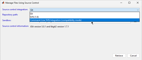
External Language Interfaces

REST Function Service: Automatic restart after MathWorks Service Host update

MATLAB REST function services rely on the MathWorks Service Host (MSH) for communication with MATLAB from client applications. MSH regularly releases updates and restarts automatically after updates are installed. If services are running before the update, the REST function connector stops during the update and then automatically restarts, along with the running services, when the MSH is available.

Any computations or requests made by your program during the update cannot be recovered. If you have long-running function calls, you can specify a preferred restart time to avoid interruption of your workflow and possible loss of data. For more information, see the PreferredRestartHour property of the RESTFunctionConnector object.

Call C++ from MATLAB: Convert MATLAB structures to C++ struct arrays when passing data from MATLAB

You can pass a MATLAB structure as a parameter to a C++ function. MATLAB converts the structure to a C++ struct argument. For more information, see Pass struct Parameter.

You can convert MATLAB structures to C++ struct arrays using the clibConvertArray function.

For information about publishing C++ functions with struct parameters that accept MATLAB structures, see Supported struct Types.

Call MATLAB from C++: Create MATLAB data arrays from user-managed buffers

You can create a MATLAB data array (MDA) using memory already allocated, without copying data or allocating extra memory, using the MATLAB Data API for C++ function createArrayFromBuffer. When you create an MDA from a buffer, you can specify a custom deleter function to manage the buffer. For more information, see Create MATLAB Data Array and Manage Memory from User-Managed Buffer.

Call MATLAB from C++: Create matlab::data::CharArray from UTF-8 input

Use the createCharArrayFromUTF8 function of the MATLAB Data API for C++ matlab::data::ArrayFactory class to create a matlab::data::CharArray object from an std::string of UTF-8 characters.

Java: Support for OpenJDK 21 Java

MATLAB now supports OpenJDK 21 Java from https://adoptium.net/. For supported version information, see MATLAB Interfaces to Other Languages.

Python: Support for CPython version 3.12

MATLAB now supports CPython version 3.12, in addition to existing support for versions 3.9, 3.10, and 3.11. For supported version information, see Versions of Python Compatible with MATLAB Products by Release.

Call Python from MATLAB: Follow Python type hints when passing data from MATLAB

MATLAB can automatically convert a floating-point integer to a Python int when passing data to a Python function. This conversion occurs if a Python type hint specifies an integer data type. For more information, see Pass MATLAB Data to Python.

Call MATLAB from Python: Convert between Python and MATLAB dictionaries

When passing data from Python to MATLAB, you can more easily convert Python dictionaries to MATLAB dictionaries. To convert a Python dict to a MATLAB dictionary, first convert the Python dict to a matlab.dictionary object, and then pass the matlab.dictionary object to MATLAB.

Additionally, MATLAB can now pass a MATLAB dictionary to Python as a matlab.dictionary object. A matlab.dictionary object behaves like a Python dict.

For more information, see Use MATLAB Dictionaries in Python.

.NET: Cross-platform support for .NET 6 and higher

In addition to existing support on Microsoft Windows platforms, MATLAB now supports .NET Runtime 6.0 and higher on macOS and Linux platforms. For more information, see System Requirements for Using MATLAB Interface to .NET.

.NET: Support for .NET 8

MATLAB now supports .NET 8, in addition to existing support for the Microsoft .NET Framework. For supported version information, see MATLAB Interfaces to Other Languages.

Compilers: Support for Intel C++ icx and Fortran ifx

MATLAB supports two additional compilers for building C and C++ interfaces, MEX files, and standalone MATLAB engine and MAT-file applications on Windows platforms.

SupportCompilerPlatform

Added

Intel oneAPI DPC++/C++ Compiler (icx)

Windows

Added

Intel Fortran Compiler (ifx)

Windows

For continued support for building your applications, consider upgrading to a supported compiler. For an up-to-date list of supported compilers, see Supported and Compatible Compilers.

Hardware Support

Arduino Hardware: Support for Arduino UNO R4 WiFi and Minima boards

You can now use the MATLAB Support Package for Arduino Hardware to communicate with the Arduino UNO R4 WiFi board over USB and WiFi and the Arduino UNO R4 Minima board over USB. Use the arduino object to connect to the two boards.

However, you cannot use the support package to interface the two boards with a servo motor, Adafruit Motor Shield V2, motor carrier, serial devices, or sensors. Also, this feature is available only when you use the MATLAB Support Package for Arduino Hardware in the installed version of MATLAB.

Arduino Hardware: Use MATLAB Support Package for Arduino Hardware in MATLAB Online through web browser

Starting in R2024b, you can use MATLAB Support Package for Arduino Hardware in MATLAB Online to communicate with Arduino hardware through your web browser. You must install the MATLAB Connector™ on your host computer to use the support package in MATLAB Online. For more information, see Get Started with MATLAB Online for Arduino.

Raspberry Pi Hardware: Support for Debian 12 Bookworm

You can now use the Raspberry Pi Blockset with boards that have the Debian 12 Bookworm Raspberry Pi operating system installed.

Raspberry Pi Hardware: libcamera support on camera boards with Bullseye and Bookworm operating systems

The libcamera packages are now installed as part of the Raspberry Pi Blockset for the Bullseye and Bookworm operating systems. The libcamera functionality is available when you enable the camera module peripheral in the Hardware Setup tool.
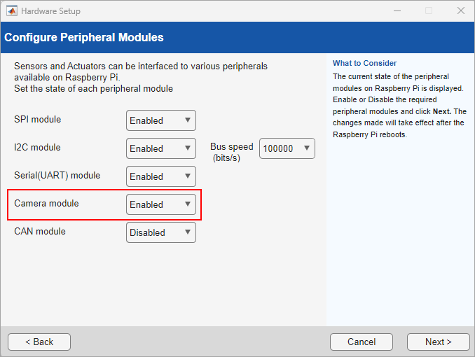
In the Hardware Setup tool, the Configure Peripheral Modules window shows the option to enable or disable the camera module.

As part of the libcamera update, the cameraboard object no longer displays the ImageEffect and VideoStabilization properties for the Bullseye and Bookworm operating systems.

Raspberry Pi Hardware: Support for Raspberry Pi 5

You can now use the Raspberry Pi Blockset with the Raspberry Pi 5 board. This support is available in the installed version of MATLAB and MATLAB Online.

However, you cannot use the Raspberry Pi 5 board with a camera board, servo motor, or pulse width modulation (PWM) signals.

Raspberry Pi Hardware: Support for Camera with Raspberry Pi 5 (December 2024 Version 24.2.3)

Starting in version 24.2.3 of Raspberry Pi Blockset, you can interface a camera board and an ArduCam multi-camera adapter module with the Raspberry Pi 5 board. This support is available for both MATLAB Online and the desktop environment.

 Functionality being removed or changed

enableI2C, disableI2C, enableSPI and disableSPI functions have been removed

Errors

These functions have been removed:

  • enableI2C

  • disableI2C

  • enableSPI

  • disableSPI

Instead, in the Hardware Setup tool, use the Configure Peripheral Modules window to enable or disable I2C and SPI interfaces on Raspberry Pi.

R2024a

New Features, Bug Fixes, Compatibility Considerations

Environment

 Editor Spell Checker: Check spelling in text and comments in MATLAB code files

In the Editor and Live Editor, you can check for spelling issues in text lines and comments. Spell checking is supported for US English in MATLAB code files (.m) and live code files (.mlx).

To enable spell checking, go to the View tab and click the Spelling button on. Words with a potential spelling issue are underlined in blue. To resolve the issue, click the word and select one of the suggested corrections. You also can choose to ignore the issue or add the flagged word to your local dictionary. To navigate between issues using the keyboard, use Alt+F7 and Alt+Shift+F7.

To remove words from your local dictionary, go to your MATLAB preferences folder (the folder returned when you run prefdir) and edit the file dict/en_US_userDictionary.tdi.

Live Editor Export: Interactively customize export options when exporting to Markdown files and Jupyter notebooks

You can interactively export live scripts and functions to Markdown files and Jupyter® notebooks and customize export options. For example, you can change the resolution and format of figures in the converted file (requires the files to be run before exporting).

To interactively export to a Markdown file or Jupyter notebook, on the Live Editor tab, click Export and select Export to Markdown or Export to Jupyter Notebook.

For more information, see Ways to Share and Export Live Scripts and Functions.

Live Editor Controls: Add date pickers to live scripts

Add a date picker to your live script to select a date interactively. To add a date picker, go to the Live Editor tab, and in the Code section, select Control > Date Picker.

Date picker with the date 25-Oct-2023 selected, assigned to the variable startDate

For more information, see Add Interactive Controls to a Live Script.

Live Editor Controls: Replace with similar controls

In live scripts, you can replace some controls with other controls that have similar functionality. For example, you can replace a check box with a state button, and a numeric slider with a numeric spinner. Replacing one control with another preserves relevant configuration values, such as range and default values.

To replace a control with another, right-click the control and select Replace with Control Name. You also can select the control in the live script, go to the Live Editor tab, click Control, and select from the available options. The Control menu shows only the controls that can replace the selected control.

For more information, see Add Interactive Controls to a Live Script.

Live Editor Tasks: Create Live Editor task class from template

You can use a template to create a Live Editor task class. To create a Live Editor task class from a template, go to the Editor or Live Editor tab and select New > Live Task Class. Customize the template and then use the matlab.task.configureMetadata function to configure the task and make it available in the Live Editor.

For more information, see Live Editor Task Development Overview.

Live Editor Output: View table, timetable, structure array, and cell array output with enhanced readability

Tables, timetables, structure arrays, and cell arrays in the output of the Live Editor have enhanced readability. The updated displays have a streamlined look, including a simplified, borderless design and row striping for easier data review and analysis.
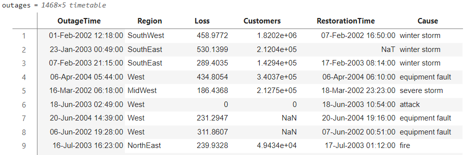
Live Editor output view of a table of power outage data with a borderless design with row striping

Find and Replace Dialog Box: Disable wrap-around search

You can disable the wrap-around search behavior in the Find and Replace dialog box using settings. To disable the wrap-around search behavior, use this code.

s = settings;
s.matlab.editor.find.WrapAround.PersonalValue = 0;
For more information including a list of additional search settings, see matlab.editor Settings.

In MATLAB Online, you also can use preferences to disable the wrap-around search behavior. On the Home tab, in the Environment section, click Preferences. Select MATLAB > Editor/Debugger > Find and Replace and in the Search behavior section, clear the Wrap around option. For more information, see Editor/Debugger Preferences.

Editor Indenting: Configure automatic indenting behavior

You can configure the behavior of automatic indenting in the Editor and Live Editor. For example, you can specify whether automatic indenting formats the entire document and whether it adds white space to empty lines.

To configure the behavior of automatic indenting, use settings. For example, enable formatting the entire document when automatic indenting is enabled.

s = settings;
s.matlab.editor.indent.SmartIndentEntireDocument.PersonalValue = 1;
For more information, see matlab.editor Settings.

In MATLAB Online, you also can use preferences to configure automatic indenting behavior. On the Home tab, in the Environment section, click Preferences. Select MATLAB > Editor/Debugger > Indenting and in the Smart indenting section, adjust the automatic indenting options as needed. For more information, see Editor/Debugger Preferences.

Editor YAML and Markdown Support: View and edit YAML and Markdown files with syntax highlighting and automatic indenting while typing

The Editor displays YAML files with syntax highlighting for keywords, variables, strings, numbers, and comments. In addition, the Editor automatically indents lines of code in YAML files while you type.

The Editor also displays Markdown files with syntax highlighting for headings, horizontal rules, lists, code blocks, comments, and other entries. You can change the syntax highlighting colors for Markdown files using settings. For example, change the color of headings in Markdown files to purple.

s = settings;
s.matlab.editor.language.markdown.HeadingColor.PersonalValue = [183 70 255];

For more information, see matlab.editor Settings.

In MATLAB Online, you also can use preferences to configure how the Editor displays YAML and Markdown files. On the Home tab, in the Environment section, click Preferences. Select MATLAB > Editor/Debugger > Other Languages and then Markdown or YAML, and adjust the options as needed.

Accessibility in MATLAB Online: Access the Command Window scroll buffer region using the keyboard

In MATLAB Online, you can access previous commands and output in the Command Window scroll buffer region using the keyboard. To enter the scroll buffer region, press Shift+Tab. The cursor moves to the last output or command. Use the up arrow and down arrow keys to move up and down between previous commands and output within the scroll buffer region. To move back to the command prompt, press Tab.

Accessibility in MATLAB Online: Use a screen reader to create and edit live scripts and functions in the Live Editor

In MATLAB Online, you can now use a screen reader to interact with live scripts and functions. When using a screen reader in a live script or function, you hear additional information about text lines, code lines, and section breaks that help provide context. For example:

  • When you are on a text line, you hear information about formatting, hyperlinks, tables, images, and equations within the line.

  • When you are on a code line, you hear the line number, content, and whether the line has output associated with it.

  • When you are on a code line containing a control or task, you hear the name of the control or task as well as its current value.

For more information, see Use a Screen Reader in MATLAB Online.

Add-Ons in MATLAB Online: Install and manage add-ons using Add-Ons panel

Use the Add-Ons panel to find, install, and manage add-ons in MATLAB Online. To open the Add-Ons panel, click the Add-Ons button in the sidebar on the left side of the MATLAB Online desktop.

For more information, see Get and Manage Add-Ons.

Cloud Storage in MATLAB Online: View your connections using Connections panel

Use the Connections panel to view and navigate to your available connections in MATLAB Online, including MATLAB Drive. To open the Connections panel, in the sidebar on the left side of the MATLAB Online desktop, click the Open more panels button (three-dot icon) and select the Connections panel.

Cloud Storage in MATLAB Online: Access your OneDrive files (June 2024)

In MATLAB Online, you can access your Microsoft OneDrive account and its contents by connecting to your account using the Connections panel. Once connected, you can view and edit your stored files and save new files to your account directly from the MATLAB Online desktop environment. For more information, see Use MATLAB Online to Access Files in Microsoft OneDrive.

Editor in MATLAB Online: Resolve conflicts with externally modified files

When saving changes to a file open in the MATLAB Online Editor, if the file has been modified outside of MATLAB, you can compare the two versions of the file before saving to avoid losing content.

Editor in MATLAB Online: Reopen last closed file

In MATLAB Online, you can reopen the last closed file in the Editor and Live Editor. To reopen the file, go to the Home tab and select Open > Reopen <filename>.

Find Files in MATLAB Online: Search for and replace text in filenames and file content

You can search for and replace text in filenames and file content using the Find Files panel in MATLAB Online. Replacing text is supported in text files (.txt) and MATLAB code files (.m).

To open the Find Files panel, click the Find Files button in the sidebar on the left side of the MATLAB Online desktop. To limit the search to only filenames or file content, click the Filters button and clear the Filename or Content within files search type.

For more information, see Find Files.

MATLAB Drive: Get recipient suggestions when sharing (April 2024)

When you share a folder using a personal invitation, MATLAB Drive suggests people to share the folder with based on who you have shared with most recently and frequently. Only people who have previously accepted an invitation from you are included in the list. You can filter the list of suggestions by entering the first name, last name, or email address of your intended recipient. For more information, see Share Folders Using MATLAB Drive.

MATLAB Drive: Updated user interface with collapsible sidebar (May 2024)

MATLAB Drive Connector is now renamed to MATLAB Connector and includes several visual updates including a new sidebar that can be collapsed when needed. For more information about MATLAB Connector, see Use MATLAB Connector to Manage Your Files.

Product Version Number: All products now use consistent version number based on release

Starting in R2023b, all products use a consistent version number based on the release. The version number includes the last two digits of the year followed by either .1 or .2, where .1 indicates an “a” release and .2 indicates a “b” release. For example, all products in R2023b have a version number of 23.2. Changes to the version number no longer indicate a major product update.

In previous releases, each individual product used a different version number. This change does not affect R2023a or earlier releases.

 Functionality being removed or changed

Form feed characters and vertical tabs display in the Editor

Behavior change

Form feed characters and vertical tabs now display in the Editor as symbols. Previously, form feed characters and vertical tabs were not displayed.
Line of code showing a form feed symbol at the beginning of the line and a vertical tab symbol at the end of the line

AcceptHTML and EmbedImages name-value arguments of the export function are false by default

Behavior change

For the export function, the default value of the AcceptHTML and EmbedImages name-value arguments is now false. Previously, the default value of the name-value arguments was true. Set AcceptHTML to true to include HTML markup when you convert live scripts or functions to Markdown files. Set EmbedImages to true to embed images and figures when you convert live scripts or functions to Markdown files or Jupyter notebooks.

Language and Programming

 Local Functions: Define functions anywhere in scripts and live scripts

Local functions can be added anywhere in scripts and live scripts except within conditional contexts, such as if statements or for loops. Each local function must begin with its own function definition statement and end with the end keyword. For more information, see Add Functions to Scripts.

createArray Function: Generate arrays of specified class and size

The createArray function enables you to create arrays of almost any MATLAB class and size. Specify a class name or prototype, a fill value, or a combination of these arguments to populate the array. For example, create a 1-by-3 array based on a complex-valued prototype of class single and a fill value of NaN.

X = createArray(1,3,Like=single(1+1i),FillValue=NaN)
X =

  1×3 single row vector

      NaN + 0.0000i      NaN + 0.0000i      NaN + 0.0000i

MATLAB Language Terminology: Packages are now called namespaces

The MATLAB language feature known as a package is now called a namespace. Namespaces are used to organize code, and in MATLAB, they are defined by folders that begin with a + symbol. As of R2024a, the terminology is updated in both the documentation and software. The behavior remains the same.

Metaclass Renaming: Metaclasses and class members have new names

In R2024a, metaclasses are contained in a new namespace, matlab.metadata. Some of the classes, properties, and methods also have new names. Their behavior remains the same.

Class Name in R2023b and EarlierNew Name as of R2024a
meta.packagematlab.metadata.Namespace
meta.classmatlab.metadata.Class
meta.propertymatlab.metadata.Property
meta.MetaDatamatlab.metadata.MetaData
meta.eventmatlab.metadata.Event
meta.methodmatlab.metadata.Method
meta.DynamicPropertymatlab.metadata.DynamicProperty
meta.EnumeratedValuematlab.metadata.EnumerationMember
meta.Validationmatlab.metadata.Validation
meta.ArrayDimensionmatlab.metadata.ArrayDimension
meta.FixedDimensionmatlab.metadata.FixedDimension
meta.UnrestrictedDimensionmatlab.metadata.UnrestrictedDimension

MATLAB will continue to recognize the old names. However, code that relies on string comparisons to identify metaclasses might need to be updated to continue to work as expected. See the Version History section on the individual class pages for more information.

Class Diagram Viewer: Show associations for classes

The Class Diagram Viewer app can now identify and display associations between classes. When the type of a class property is explicitly defined as another class using class validation, the Class Diagram Viewer can show this association by connecting the property to the class card of its type with an arrow. Use the Associations check box in the toolstrip of the app or the ShowAssociations property of matlab.diagram.ClassViewer to toggle associations on and off in the diagram.

Class Constructor: .?MyClass syntax accepts immutable properties as name-value arguments

In previous releases, the .?MyClass syntax could be used in functions and methods to accept class properties as name-value arguments, but the syntax did not work with immutable properties. To enable immutable properties to be set as name-value arguments, you had to use a separate struct in the arguments block. For example, opts.?ExampleClass could handle Prop2 and Prop3, but a separate struct, opts.Prop1, was required for Prop1.

classdef ExampleClass
    properties (SetAccess=immutable)
        Prop1
    end
    properties (SetAccess=public)
        Prop2
        Prop3
    end
   
    methods
        function obj = ExampleClass(opts)
            arguments
                opts.Prop1
                opts.?ExampleClass
            end
        end
    end
end

Starting in R2024a, opts.?ExampleClass works with immutable properties as well, so you no longer need to handle Prop1 separately. This syntax for using immutable properties as name-value arguments only works in the class constructor.

MATLAB backgroundPool Function: save function supported in background threads

Use the save function in thread-based environments, including the MATLAB backgroundPool. Saving Version 7.3 MAT-files is not supported.

hasActiveValue Function: Verify that setting has active value

The hasActiveValue function returns a logical value indicating whether a given setting currently has an active value. For example, this code checks if the maximum width setting for comments has an active value. If it does not, it sets the personal value for the setting, which also updates the active value.

s = settings;
if ~hasActiveValue(s.matlab.editor.language.matlab.comments.MaxWidth)
    s.matlab.editor.language.matlab.comments.MaxWidth.PersonalValue = 80   
end

MATLAB Debugger: View private, protected, and hidden class property values using display and details

The MATLAB debugger now offers additional access to private, protected, and hidden class properties and their values using the display and details functions. For example, set a breakpoint at the end of the incPrivateProp method of the DebugDemo class.

classdef DebugDemo
    properties
        PublicProp = 0
    end
    properties (Access=private)
        PrivateProp = 0
    end
    methods
        function obj = incPrivateProp(obj)
            obj.PrivateProp = obj.PrivateProp + 1;
        end
    end
end

Construct an instance test of the DebugDemo class, then call the incPrivateProp method.

test = DebugDemo;
test.incPrivateProp

Once you enter the debugger at the breakpoint, calling display on the object returns public properties and their values.

K>> obj % Or display(obj)
obj = 

  DebugDemo with properties:

    PublicProp: 0

  Show all accessible properties of DebugDemo

Click the Show all link to show all properties and values, including private, protected, and hidden properties.

     PublicProp: 0
    PrivateProp: 1

   Open Class Diagram Viewer for DebugDemo

Calling details on the object also shows all properties and values, including private, protected, and hidden properties.

K>> details(obj)
 Debug view of DebugDemo with properties:

     PublicProp: 0
    PrivateProp: 1

  Methods

Function Input Arguments: Automatically add input arguments to arguments block

When you complete an arguments block using automatic suggestions and completions, MATLAB automatically adds an entry for each input argument in the function declaration as well as an end keyword at the end of the block.

Validation Functions: mustBeUnderlyingType accepts multiple data types

mustBeUnderlyingType now accepts multiple data types for the typenames input argument.

 Functionality being removed or changed

Some matlab.diagram.ClassViewer member names have changed

Behavior change

MATLAB now refers to packages as namespaces. Several members of matlab.diagram.ClassViewer have been renamed to reflect this terminology change. Their behavior remains the same.

Member Name in R2023b and EarlierNew Name as of R2024a
Constructor: Packages name-value argumentNamespaces
Constructor: IncludeSubpackages name-value argumentIncludeInnerNamespaces
Property: ShowPackageNamesShowNamespace
Method: importClassesFrom, Packages name-value argumentNamespaces
Method: importClassesFrom, IncludeSubpackages name-value argumentIncludeInnerNamespaces

Negating a matlab.lang.OnOffSwitchState enumeration member preserves class

Behavior change

Before R2024a, negating a matlab.lang.OnOffSwitchState enumeration member returned a logical value. MATLAB now preserves the class of matlab.lang.OnOffSwitchState members when you negate them. See matlab.lang.OnOffSwitchState for more information.

Change to precedence for constructors in class folders

Warns

When a class and a function on the path have the same name, MATLAB currently gives precedence to the class constructor if the class is defined inside a class folder (@-folder). The constructor takes precedence even if the function appears before the class on the path.

In a future release, this precedence rule will be removed. In other words, if a function appears before a class of the same name on the path, the function will have precedence regardless of whether the class is defined in a class folder. To give precedence to the class constructor, update your path configuration. To give precedence to the other function, remove the class from the path or rename one of the conflicting items. MATLAB currently displays a warning when a name is resolved to a class constructor instead of a function earlier on the path. For more information, see Precedence of Classes in @-folders over Functions of the Same Name Will Be Removed in a Future Release.

Defining classes and namespaces: Using schema.m will not be supported in a future release

Still runs

Support for classes and namespaces defined using schema.m files will be removed in a future release. Replace existing schema-based classes with classes defined using the classdef keyword.

MATLAB Identifiers: The maximum length of MATLAB identifiers will increase in a future release

Behavior change in future release

The maximum length of MATLAB identifiers will increase in a future release. This change allows variables, functions, classes, and many other entities to have names that exceed 63 characters. Code that depends on identifiers having a maximum length of 63 characters may no longer run as expected.

MATLAB Scripts: Scripts without executable code will now error

Behavior change

Scripts without executable code will now error. For example, the following script contains no executable code:

% this is a script file 
; 

function foo 
end

Prior to R2024a this script would be considered valid. In R2024a, attempting to run this script would result in an error being thrown.

Data Analysis

islocalmax2 and islocalmin2 Functions: Find local extrema in two dimensions

Find local maxima or minima and the prominence of each extremum in two-dimensional data sets using the islocalmax2 or islocalmin2 function, respectively.

clip Function: Clip values to specified range

Clip the values in an array, table, or timetable to a specified range using the clip function. clip replaces values less than the lower bound with the lower bound value and replaces values greater than the upper bound with the upper bound value.

When clipping table or timetable data, you can:

  • Specify tabular variables to clip by using the DataVariables name-value argument.

  • Append or replace tabular variables with variables containing clipped data by using the ReplaceValues name-value argument.

mean and median Functions: Compute weighted statistics

Compute the weighted mean or the weighted median of input data by specifying the Weights parameter of the mean or median function, respectively.

iqr Function: Return first and third quartiles

The iqr function can now return the first and third quartiles of the input data by using a second output argument q. The first element of q along the smallest operating dimension is the first quartile of the input data, and the second element of q along the smallest operating dimension is the third quartile.

Experiment Manager: Apply and reset filters for numeric, character array, and string variables in results table

In the Experiment Manager app, you can apply or reset a filter for a variable in the results table. Select Filters in the toolstrip and configure the corresponding section of the Filters pane. Set the bounds for a numeric variable, or specify the contents of a character array or string variable. Previously, you could apply a filter only to numeric variables and you could not reset the numeric filter.
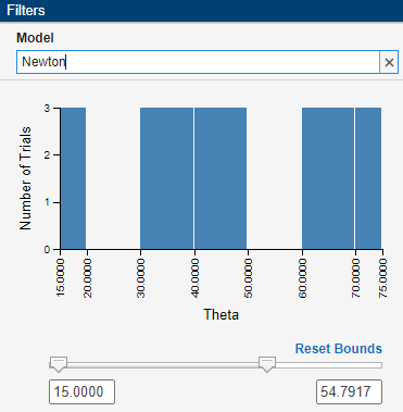
Filters pane in Experiment Manager. A string filter for the value "Newton" is applied for the Model parameter, and a numeric filter for values less than 54.7917 is applied for the Theta parameter.

Experiment Manager: Add supporting files

In the Experiment Manager app, add files required by your experiment using the Supporting Files section of the experiment definition tab.

After you run an experiment, the Detected Files section lists detected supporting files. If Experiment Manager does not detect some of your supporting files, your trials will produce an error. You can manually select files to include by clicking Add in the Additional Files section. You can also update the Detected Files section by clicking Refresh.

Live Editor Output: View sparklines and summary statistics for tables

For tables or timetables in the output of the Live Editor, you can display sparklines and summary statistics to quickly visualize and interpret the data in each variable.

To display sparklines or summary statistics, right-click the table and show sparklines or summary statistics using the context menu. To show more information related to specific points, point to a sparkline.
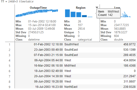
Live Editor output view of a timetable of power outage data with a sparkline and summary statistics for each table variable. A tooltip for the Region variable sparkline indicates that there are 142 outages in the MidWest region.

Smooth Data Live Editor Task: Return moving window size

The Smooth Data task in the Live Editor can now return the moving window size. If you specify the moving window size, the returned window size matches the input value. If you do not specify the moving window size, then the returned window size is heuristically determined based on the input data. If the moving window is asymmetric, then the returned window is a two-element vector of nonnegative integers [b f], where the window contains the current element, b elements backward, and f elements forward.

fillmissing and filloutliers Functions: Define missing or outlier locations using table

Define the locations of missing entries or outliers using a table. Specify the MissingLocations name-value argument of the fillmissing function or the OutlierLocations name-value argument of the filloutliers function.

Previously, fillmissing and filloutliers supported only array indicators for missing entries or outliers.

Group-Wise Computations: Apply multiple binning methods to grouping variable

For these functions, apply multiple binning methods to one grouping variable or vector by specifying a cell array of binning methods.

datetime Data Type: Specify time zone offset using duration value

You can specify a time zone offset for a datetime array by using a duration value.

To specify an offset when you use the datetime function, specify the TimeZone name-value argument.

t = datetime("now",TimeZone=hours(5))

To specify an offset after you create a datetime array, assign the offset to its TimeZone property.

t = datetime("now")
t.TimeZone = hours(5)

categories Function: Return list of categories as categorical array or string array

When using the categories function, you can specify the OutputType name-value argument to return the list of categories as a categorical array or string array. By default, the function returns the list of categories as a cell array of character vectors.

Unstack Table Variables Live Editor Task: Generate template code for custom aggregation function

In the Unstack Table Variables Live Editor Task, when you select the Custom function option for the Aggregator for new table variable values method, you can generate template code that can help you write your own custom aggregation function.

  1. Select Custom function.

  2. Select Local function from the next menu.

  3. Click New to add a new local function to the script.

  4. Select the name of the new local function from the next menu.

The Live Editor task generates template code and places it within the live script. To customize this code, edit it in the live script.

Data Import and Export

 Secrets in MATLAB Vault: Remove sensitive information from code

You can remove sensitive information, such as passwords, from code by using secrets and a local MATLAB vault. Your MATLAB vault is accessible only from the exact combination of your operating system account and local machine. Removing sensitive information increases the security of your code and allows you to share your code more easily. Create and manage secrets in your vault using these new functions:

  • setSecret – Move sensitive information into a secret in your vault.

  • getSecret – Retrieve a secret from your vault.

  • isSecret – Determine if a secret exists in your vault.

  • removeSecret – Remove a secret from your vault.

  • setSecretMetadata – Set the metadata of a secret in your vault.

  • getSecretMetadata – Retrieve the metadata of a secret in your vault.

  • listSecrets – Display the names and metadata of all the secrets in your vault.

SFTP: Specify remote current working folder at login

When you connect to an SFTP server using the sftp function, you can specify a remote current working folder by using the StartingFolder name-value argument.

openedFiles Function: Get file identifiers of all open files

Get the file identifiers of all open files using the openedFiles function.

HDF5 Interface: Import HDF5 data using Import Tool in MATLAB Online and Import Data Live Editor task

You can import HDF5 data by using the Import Tool app in MATLAB Online or by using the Import Data Live Editor task in live scripts. Using these options, you can:

  • Visualize the structure and contents of HDF5 data interactively.

  • Search for specific groups, datasets, and attributes.

  • Graphically select and deselect groups, datasets, and attributes to import.

  • Generate reusable MATLAB code to import HDF5 data.

HDF5 Interface in MATLAB Online: Import HDF5 data by double-clicking HDF5 files

You can open the Import Tool app to import HDF5 data by double-clicking an HDF5 file in MATLAB Online.

Serial and TCP/IP Connections: Label and Find Connections

You can use the following functions to find existing serialport and tcpclient connections and return object handles for these connections.

These commands can return all existing connections of the respective type or only those connections having specified property values. In particular, each interface has a new Tag property that you can use to label and find connections. For instance, the following command finds existing serialport connections whose Tag property is "Scope".

S = serialportfind(Tag="Scope");

Such tags are useful when you create a connection in one function and use a different function to perform operations on the connection.

Image File Format Libraries: LibTIFF library upgraded to version 4.6.0

The LibTIFF library is upgraded to version 4.6.0.

Scientific File Format Libraries: HDF4 library upgraded to version 4.2.16.2

The HDF4 library is upgraded to version 4.2.16.2.

Scientific File Format Libraries: HDF5 library upgraded to version 1.10.11

The HDF5 library is upgraded to version 1.10.11.

 Functionality being removed or changed

fopen("all") syntax will be removed

Warns

The fopen("all") syntax will be removed in a future release. To get the file identifiers of all open files, use the openedFiles function instead.

Mathematics

 ode Object: Solve ODEs and perform sensitivity analysis using SUNDIALS solvers

ode objects support three new values for the Solver property: "cvodesStiff", "cvodesNonStiff", and "idas". The new solvers provide access to a subset of the SUNDIALS suite of differential equation solvers.

  • Adjust the values of InitialStep, MaxStep, and MaxOrder used by the new solvers with the SolverOptions property of the ode object.

  • Examine how sensitive the equations are to variations in parameter values using sensitivity analysis, supported only by the new SUNDIALS solvers. To perform sensitivity analysis, set the Sensitivity property of the ode object using an odeSensitivity object.

pagelsqminnorm Function: Calculate minimum-norm least-squares solutions to systems of linear equations in N-D arrays

Calculate the minimum-norm least-squares solutions to the systems of linear equations defined by N-D arrays using the pagelsqminnorm function. In this context, the N-D arrays are treated as containers for several 2-D matrices.

pagepinv Function: Calculate Moore-Penrose pseudoinverses of pages of N-D array

Calculate the Moore-Penrose pseudoinverses of the pages of an N-D array using the pagepinv function. In this context, the N-D array is treated as a container for several 2-D matrices.

scatteredInterpolant Object: Extend interpolation boundary into extrapolation domain

When using scatteredInterpolant, you can specify the extrapolation method as "boundary". The "boundary" extrapolation method extends the values on the scatteredInterpolant interpolation boundary into the extrapolation domain. This method mitigates extreme extrapolation values and maintains continuity between the extrapolation and interpolation domains.

polydiv Function: Divide polynomials using long division

Use the polydiv function to divide two polynomials using long division.

The syntax [q,r] = polydiv(b,a) is equivalent to deconvolving vector a out of vector b using the polynomial long division method, such that b = conv(a,q) + r. However, using polynomial long division to find deconvolutions can result in numerically unstable results. For more numerically stable computations when finding the deconvolutions, use the least-squares method instead, as provided in the deconv function.

polyfit Function: Return R-squared value

The error estimation structure S, returned as an optional second output of the polyfit function, contains a new field named rsquared. rsquared is the coefficient of determination, or (unadjusted) R-squared value. Use S with the polyval function to obtain error estimates.

polyshape Object: Control when union and intersect methods simplify output

You can control when the union and intersect methods of polyshape simplify their output by specifying the new Simplify name-value argument, which can be either true (default) or false. By default, the methods return a well-defined polygon by resolving boundary intersections and improper nesting and also remove duplicate points and degeneracies. However, you can specify Simplify=false to gain performance when performing a series of unions or intersections. In this case, you can simplify the output once at the end either by specifying Simplify=true in the final method call or by using the simplify method on the final output polygon.

spdiags Function: Specify diagonal elements as matrix, vector, or scalar

The spdiags function now supports implicit expansion for the diagonal elements argument Bin. You can specify the diagonal elements as a matrix, vector, or scalar, and the function expands the values if the argument is specified as a vector or scalar.

Before R2024a, you can replace the diagonal elements of m-by-n matrix A with the columns of a matrix Bin only if Bin has at least min(m,n) rows. Starting in R2024a, the spdiags function accepts the Bin argument as a matrix, vector, or scalar.

sub2ind Function: Specify subscript inputs as scalars and vectors

The sub2ind function now supports scalar expansion and accepts a mix of scalars and vectors for subscript inputs. For example, sub2ind(sz,[1 2 3],2) is now the same as sub2ind(sz,[1 2 3],[2 2 2]). Previously, the subscript inputs were required to be the same size.

 Functionality being removed or changed

colon operator will no longer support nonscalar operands

Warns

colon now issues a warning when creating vectors if one or more operands are not scalar. For example, expressions like [1 2 3]:2:10 now warn. This warning will become an error in a future release, removing support for nonscalar operands. Previously, colon used the first element of any nonscalar operands to evaluate the expression.

Graphics

fpolarplot Function: Plot mathematical expressions in polar coordinates

Plot mathematical expressions in polar coordinates by using the fpolarplot function. This function replaces the ezpolar function.

Plot of a function in polar coordinates

Polar Plots: Create filled regions in polar coordinates

Create different types of filled regions in polar coordinates using the thetaregion, radiusregion, and polarregion functions. Filled regions are useful for highlighting one or more sections of a plot.
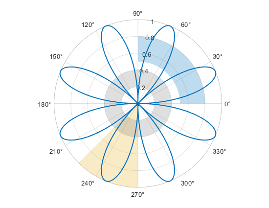
Polar plot with three filled regions

linestyleorder Function: Control line styles when plotting multiple data series

Control the line styles of your plots by using the linestyleorder function. When you call this function, MATLAB uses the specified line styles for any new plots you create, and it updates the existing plots in the specified figure or axes.
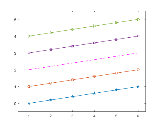
Five plotted lines that each have a different line style and marker combination

rgb2hex and hex2rgb Functions: Convert between RGB triplets and hexadecimal color codes

Use the rgb2hex function to convert RGB triplets to hexadecimal color codes. Use the hex2rgb function to convert hexadecimal color codes to RGB triplets. Both functions support RGB values as normalized single and double values as well as 8- and 16-bit unsigned integer values. Both functions also support three- and six-digit hexadecimal codes.

Quiver Plots: Access the multiplier used to scale arrows

Query the ScaleFactor property of a Quiver object to access the value that MATLAB uses to scale the magnitudes of the arrows in your plot. The scale factor is useful when you want to maintain the scale between the arrows and other graphics objects in the axes.

Legends and Rectangles: Control transparency of legend boxes and rectangle faces

You can control the transparency of legend boxes and rectangles:

  • Control the background transparency of a legend box by setting the BackgroundAlpha property of the Legend object to a value between 0 (completely transparent) and 1 (opaque).

  • Control the transparency of a rectangle by setting the FaceAlpha property of the Rectangle object to a value between 0 and 1.

A semitransparent legend that overlaps with several plotted lines and two overlapping, semitransparent rectangles

ConstantLine and ConstantRegion Objects: Layer reference lines and filled regions in plots

You can move ConstantLine objects (created with xline and yline) and ConstantRegion objects (created with xregion and yregion) above or below other elements in a plot by setting the Layer property to "top" or "bottom".
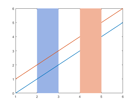
Two plotted diagonal lines and two opaque regions. The first region appears behind the lines between x=2 and x=3. The second region appears in front of the lines between x=4 and x=5.

Bar Charts: Control bar group width

Control the bar group width by setting the GroupWidth property of at least one Bar object in the axes.
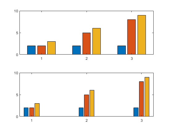
Two bar charts that display the same data, each with three groups of bars. The first chart has the default bar width and spacing between the groups. The second chart has narrower bars and wider spacing between the groups.

Donut and Pie Charts: Label charts in different ways

You can use additional properties to label donut charts and pie charts:

  • Create a large center label in a donut chart by setting the CenterLabel property of the chart. You can control the font size of the label by setting the CenterLabelFontSize property.

  • Select different labeling schemes for a donut or pie chart by setting the LabelStyle property of the chart. You can choose from six different styles, including "name", which displays slice names, and "namedata", which displays the slice names and data values.
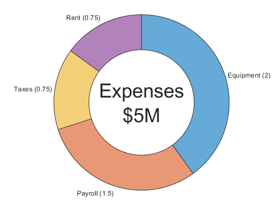
Donut chart that has a center label and slice labels that include the slice names and the corresponding data values

DatetimeRuler Object: Specify date format for secondary labels when plotting datetime data

When you plot datetime data, you can specify the format of the secondary label of the datetime ruler by setting the SecondaryLabelFormat property of the DatetimeRuler object. For example, a value of "yyyy" displays a four-digit year.

clf, cla, and clim Functions: Pass array of objects as input

Clear multiple figures or axes, or set the color limits of multiple axes at once by passing an array of objects to the clf, cla, and clim functions.

hold, axis, box, and grid Functions: Pass OnOffSwitchState values as input

Before R2024a, you could set the state of certain axes properties by passing "on" and "off" values to the hold, axis, box, and grid functions. Now, those functions accept any OnOffSwitchState values, including 0, 1, false, and true. A value of true or 1 is equivalent to "on", and a value of false or 0 is equivalent to "off".

scatterhistogram Function: Display smooth marginal histograms using kernel density estimates

Using the scatterhistogram function, you can create a scatter plot with marginal kernel density histograms by specifying the HistogramDisplayStyle name-value argument as "smooth". Previously, kernel density estimation required a Statistics and Machine Learning Toolbox™ license.

Graphics in MATLAB Online: Export graphics with specific dimensions and padding

Specify the width, height, padding, and whether to preserve the aspect ratio of the original graphic when you call the exportgraphics function.

Use these name-value arguments to control these aspects of the content:

  • Width and Height — Specify the width and height of the output.

  • Padding — Specify the amount of padding around the perimeter of the graphic.

  • Units — Specify the units for the width, height, and padding values.

  • PreserveAspectRatio — Specify whether to automatically add padding to preserve the original aspect ratio if the Width and Height values conflict with the original aspect ratio of the graphic.

 Functionality being removed or changed

ezpolar is not recommended

Still runs

The ezpolar function is not recommended. However, there are no plans to remove the function. To plot a mathematical expression in polar coordinates, use the fpolarplot function instead.

The benefits of using the fpolarplot function include:

  • A more accurate visual representation of your function. Unlike ezpolar, fpolarplot adds more function evaluation points as needed.

  • An argument for customizing the line style, marker symbol, and color.

  • A PolarAxes object, which you can customize by setting PolarAxes properties. For example, you can change the range of angle values or choose whether to display angles in radians or degrees.

This table shows some typical usages of ezpolar and how to update your code to use fpolarplot instead. To display the plotted expression as ezpolar does, use the title function.

Not RecommendedRecommended

ezpolar(@(t) cos(t))
or
ezpolar('cos(t)')

fpolarplot(@(t) cos(t))

ezpolar(@(t) cos(t),[0 pi/4])
or
ezpolar('cos(t)',[0 pi/4])

fpolarplot(@(t) cos(t),[0 pi/4])

datetick is not recommended

Still runs

The datetick function is not recommended. However, there are no plans to remove the function.

Instead of using datetick, plot datetime or duration values with any plotting function. Then you can configure the tick labels using the xtickformat and ytickformat functions or customize other aspects of your plot by setting properties of the DatetimeRuler object. For example, you can display datetime values in a variety of formats, include a time zone, or display a time zone offset.

hgexport will be removed

Still runs

The hgexport function will be removed in a future release. To save the contents of a plot as an image or vector graphics file, use the exportgraphics function. This function has a variety of options for controlling the output. For example, you can capture plots with tight cropping around the axes, control image resolution, embed fonts in PDFs, or create multipage PDFs and animated GIFs.

To save the contents of an app as an image file, use the exportapp function.

colordef, graymon, and whitebg will be removed

Warns

The colordef, graymon, and whitebg functions issue a warning that they will be removed in a future release.

axis function will no longer support outputs of limit selection mode, visibility, and y-axis direction

Warns

This syntax of the axis function, which returns the axis limit selection mode (m), visibility (v), and y-axis direction (d), issues a warning that it will be removed in a future release.

[m,v,d] = axis('state')

You can get the same information by querying these Axes properties:

In apps, plots with high marker density look different without hardware-accelerated graphics

Behavior change

When you create a plot that has a high density of markers in an app or in MATLAB Online using a system that does not have hardware-accelerated graphics, the plot displays fewer markers compared to previous releases. This change helps to maintain responsiveness during plot interactions. This change affects only a subset of systems that do not meet the recommended requirements for running MATLAB.

Here is a plot of 100,000 points on a system without hardware-accelerated graphics in R2023b and R2024a.
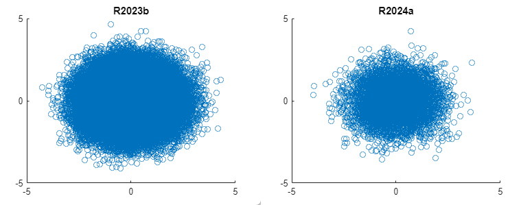
Comparison of dense scatter plots created without hardware-accelerated graphics in R2023b and R2024a. In R2024a, the plot displays fewer markers.

App Building

uicolorpicker Function: Add and configure color picker components in apps

To create a color picker in an app, use the uicolorpicker function or, in App Designer, drag a color picker UI component from the Component Library onto the canvas.
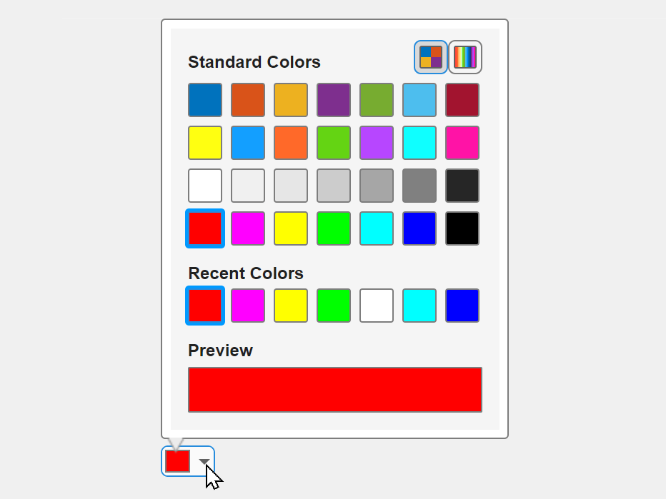
Color picker UI component showing standard colors, recent colors, and a color preview. The current color selection is red.

uislider Function: Specify step size for range slider

When you create a range slider component using the uislider function, you can specify the amount that the value changes when a user interacts with the slider thumbs by setting the Step property.

For more information, see RangeSlider Properties.

uiradiobutton Function: Specify HTML markup and display equations in radio button text

Enable text markup for radio buttons created using the uiradiobutton function by setting the Interpreter property. Specify the interpreter as "html", "latex", "tex", or "none". Specifying an interpreter is supported only in App Designer apps and in figures created with the uifigure function.

For more information, see RadioButton Properties.

uitable Function: Specify table colors using hexadecimal color codes or color names

When modifying colors in a table UI component using the BackgroundColor property, you can specify colors as hexadecimal color codes or color names, in addition to RGB triplets.

For more information, see Table Properties.

uitable Function: Visually identify table cells that have drop-down list editor

When you create a table UI component with editable cells that display categorical data, the cells include a visual indicator that the data can be edited using a drop-down list.
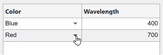
Table UI component with two columns, Color and Wavelength. The cells in the Color column have an upside-down triangle icon at the far right.

For more information about how data appears in a table UI component, see Format Tabular Data in Apps.

UI Figure Key-Press Callbacks: Access data about pressed key for larger list of keys

When you use a key-press callback, such as a KeyPressFcn or WindowKeyReleaseFcn callback, for a figure created using the uifigure function, the Character property of the callback event data can return an expanded set of keys using the Unicode® symbol for the pressed key. This change provides key data for a larger set of keyboard keys across many writing systems.

For more information, see UI Figure Properties.

App Designer: Build apps that interface with Simulink models

Interactively build a custom app that interfaces with a Simulink model by using App Designer. Use the App Designer design environment to:

  • Perform common simulation tasks from the app, such as starting and stopping the simulation and viewing simulation progress, using Simulink UI components.

  • Tune model variables from the app while the simulation runs by connecting UI components to variables.

  • Visualize simulation signals in the app by connecting signals to a time scope UI component.

For more information, see Create App for Simulink Model (Simulink).

App Designer: Convert between additional similar UI components

To convert one type of UI component to another with similar functionality, right-click the component on the canvas or in the Component Browser and select Replace With. Then, select the component to convert to. Replacing one component with another preserves relevant property values, such as font properties and callbacks that exist for both components. For example, you can now convert component types within these additional groups:

  • Push button and state button

  • Tree and check box tree

  • List box, drop-down component, and discrete knob

App Designer: Configure grid layout using improved editor interactions

Use the grid layout manager in Design View with improved interactions to more efficiently add, remove, and manage the size of multiple grid rows and columns. For more information, see Use Grid Layout Managers in App Designer.

App Designer in MATLAB Online: Access toolstrip actions and Help Center resources using search

In MATLAB Online, you can now use the Search box in the top-right corner of App Designer to easily access toolstrip actions and Help Center resources such as functions, examples, and answers.

For example, to show the background grid on the App Designer canvas, enter the word grid in the Search box. In the list of results, select the Grid toolstrip action.
Search box containing the word grid and a list of search results including toolstrip actions, functions, and examples

Axes Interactions: Customize behavior of interactions

For polaraxes and geoaxes objects created in App Designer or in figures created using the uifigure function, you can customize the behavior of axes interactions. Customize the behavior of data tips by using the InteractionOptions property of a polaraxes or geoaxes object. For geoaxes objects, you can also customize the panning and zooming behavior, as well as how to restore views, by using the same property. For more information, see PolarAxesInteractionOptions Properties and GeographicAxesInteractionOptions Properties.

Axes Interactions: Interact with axes using the keyboard

You can pan, zoom, and rotate the view of axes using the keyboard. For example, when the pan interaction is enabled on axes with focus, you can pan the view of the axes using the arrow keys. For more information, see panInteraction, zoomInteraction, and rotateInteraction.

App Testing Framework: Perform scroll gestures on axes and UI axes

You can use the scroll method to test scroll gestures on axes and UI axes. Specify the direction of the scroll gesture to mimic a user scrolling up, down, left, or right.

App Testing Framework: Perform gestures on hyperlinks

You can use the press and chooseContextMenu methods to perform gestures on hyperlink components. For example, create a hyperlink and programmatically click it to open a URL.

fig = uifigure;
hlink = uihyperlink(fig);
hlink.Text = "MathWorks";
hlink.URL = "https://www.mathworks.com/";

testCase = matlab.uitest.TestCase.forInteractiveUse;
testCase.press(hlink)

 App Testing Framework: Node expanded callback executes when gestures programmatically expand tree nodes

To better mimic a user who must expand tree nodes to interact with a nested node, the node expanded callback executes when you perform a gesture on a collapsed tree node by using the choose or chooseContextMenu method. You can specify the callback by setting the NodeExpandedFcn property of the tree.

For example, perform a choose gesture on a nested node in a tree, and display the text of any programmatically expanded nodes.

fig = uifigure;
t = uitree(fig);
t.NodeExpandedFcn = @(src,event) disp(event.Node.Text);

parent = uitreenode(t,"Text","Runners");
child1 = uitreenode(parent,"Text","Joe");
child2 = uitreenode(parent,"Text","Linda");

testCase = matlab.uitest.TestCase.forInteractiveUse;
testCase.choose(child2)
 Compatibility Considerations

If you do not want the callback to execute, preserving the behavior in R2023b and earlier, expand the tree node before performing the gesture. In this code, the callback does not execute.

fig = uifigure;
t = uitree(fig);
t.NodeExpandedFcn = @(src,event) disp(event.Node.Text);

parent = uitreenode(t,"Text","Runners");
child1 = uitreenode(parent,"Text","Joe");
child2 = uitreenode(parent,"Text","Linda");

testCase = matlab.uitest.TestCase.forInteractiveUse;
expand(parent)
testCase.choose(child2)

 Functionality being removed or changed

In apps, plots with high marker density look different without hardware-accelerated graphics

Behavior change

When you create a plot that has a high density of markers in an app or in MATLAB Online using a system that does not have hardware-accelerated graphics, the plot displays fewer markers compared to previous releases. This change helps to maintain responsiveness during plot interactions.

Note

This change only affects a subset of systems that do not meet the recommended requirements for running MATLAB.

Here is a plot of 100,000 points on a system without hardware-accelerated graphics in R2023b and R2024a.
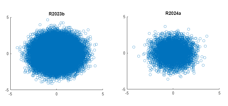
Scatter plots of the same 100,000 points in R2023b and R2024a. The R2023b plot displays more markers than the R2024a plot does.

Performance

datetime Format Parsing: Improved performance when parsing common numeric formats

datetime format parsing performance is significantly faster when parsing some common formats. In general, performance is best for text timestamps in formats that use only numeric specifiers, such as the ISO 8601 format. This list shows a few examples of such formats, which are part of ongoing efforts to improve datetime format parsing performance:

  • uuuu-MM-dd and yyyy-MM-dd

  • MM/dd/uuuu and MM/dd/yyyy

  • uuuu-MM-dd'T'HH:mm:ss.SSS'Z' and yyyy-MM-dd'T'HH:mm:ss.SSS'Z'

For example, this code creates and then parses a string array that contains a series of dates. The dates in the string array have the uuuu-MM-dd numeric format. The datetime function recognizes the format, parses the strings, and returns datetime values. The code is about 16x faster than in the previous release.

function timingTest
   d1 = datetime(2024,1,1:10000);
   s = string(d1,"uuuu-MM-dd");

   for i = 1:100
       d2 = datetime(s); 
   end
end

The approximate execution times are:

R2023b: 3.13 s

R2024a: 0.19 s

The code was timed on a Windows 11, AMD EPYC 74F3 24-Core Processor @ 3.19 GHz test system using the timeit function.

timeit(@timingTest)

imread and imwrite Functions: Improved performance with JPEG files

The imread and imwrite functions show improved performance when working with JPEG files. For example, this code reads a large JPEG image. The code is about 1.5x faster than in the previous release.

function t = imreadTimingTest
    filename = "world.topo.bathy.200407.3x21600x21600.C1.jpg";
    url = "https://eoimages.gsfc.nasa.gov/images/imagerecords/73000/73751/" + filename;
    websave(filename,url);

    f = @() imread(filename);

    t = timeit(f);
end

The approximate execution times are:

R2023b: 6.6 s

R2024a: 4.3 s

This code writes a large JPEG image. The code is about 1.6x faster than in the previous release.

function t = imwriteTimingTest
    filename = "world.topo.bathy.200407.3x21600x21600.C1.jpg";
    url = "https://eoimages.gsfc.nasa.gov/images/imagerecords/73000/73751/" + filename;
    A = imread(url);

    f = @() imwrite(A,filename);

    t = timeit(f);
end

The approximate execution times are:

R2023b: 38.3 s

R2024a: 23.8 s

The code was timed on a Windows 11, Intel Xeon Gold 6246R CPU @ 3.40 GHz test system by calling the imreadTimingTest and imwriteTimingTest functions.

smoothdata2 and fillmissing2 Functions: Improved performance for moving average methods

The smoothdata2 and fillmissing2 functions show improved performance when you specify the "movmean", "movmedian", or (for smoothdata2) "gaussian" moving method. The performance improvement is more significant when the input data has at least several hundred elements.

For example, this code smooths a 100-by-100 matrix of noisy data using the median over a 3-by-3 moving window. The code is about 3.6x faster than in the previous release.

function timingSmoothdata2 
A = rand(100,100);
for k = 1:700
   smoothdata2(A,"movmedian",3);
end
end

The approximate execution times are:

R2023b: 1.05 s

R2024a: 0.29 s

The code was timed on a Windows 11, AMD EPYC 74F3 24-Core Processor @ 3.19 GHz test system using the timeit function.

timeit(@timingSmoothdata2)

mldivide Function: Improved performance with tridiagonal matrices

The mldivide function shows improved performance when solving linear systems A*x = b with a full tridiagonal coefficient matrix A. For example, this code solves a linear system specified for tridiagonal matrix D. The code is about 6.5x faster than in the previous release.

function t = timingTest
n = 5e3;
A = randn(n);
[L,D,P] = ldl(A,"upper");
b = randn(n,1);

f = @() D\b;
t = timeit(f);
end

The approximate execution times are:

R2023b: 0.13 s

R2024a: 0.02 s

The code was timed on a Windows 11, AMD EPYC 74F3 24-Core Processor @ 3.19 GHz test system by calling the timingTest function.

audioplayer Function : Improved performance with longer duration audio signals

The audioplayer function shows improved performance when operating on audio signals longer than 100 seconds. For example, this code creates an audio player for a 300-second audio signal using a sample rate of 48 KHz. The code is about 6.1x faster than in the previous release.

function timingTest 
   Fs = 48000; 
   audioSignal = rand(300*Fs,1); 
   audioplayer(audioSignal,Fs);
end

The approximate execution times are:

R2023b: 61.9 s

R2024a: 10.1 s

The code was timed by calling the audioplayer function. Because MATLAB Online is hosted, performance is independent of the computer hardware used to access it.

Files Panel in MATLAB Online: Improved performance when previewing large MAT-files

The Files panel shows improved performance when previewing a large MAT-file in MATLAB Online. The delay between clicking the Preview button and the preview being ready is reduced.

For example, create a large MAT-file in MATLAB Online. Then, pause on the MAT-file name in the Files panel and click the Preview button that appears. You can view the MAT-file preview 5.6x sooner than in the previous release.

x = randn(50000000,1);
save sample.mat -v7.3

The approximate rendering times are:

R2023b: 14 s

R2024a: 2.5 s

Because MATLAB Online is hosted, performance is independent of the computer hardware used to access it.

Workspace Panel in MATLAB Online: Improved performance when loading large number of variables

The Workspace panel shows improved performance when loading a large number of variables in MATLAB Online. The delay between loading a MAT-file that contains a large number of variables, such as one created by a Simulink model, and the Workspace panel showing the variables is reduced.

For example, create a MAT-file that contains 2000 scalar variables using a local function.

function createVariables
for i = 1:2000
    varName = sprintf('var%d',i);
    eval([varName '=i;']);
end
save("largeFile.mat");
end

After clearing any existing variables from the workspace, load variables from the file into the workspace. In R2023b, the Workspace panel takes about 3.5 seconds to load the variables. In R2024a, you can view the variables in the Workspace panel almost instantaneously.

createVariables
load("largeFile.mat")

Because MATLAB Online is hosted, performance is independent of the computer hardware used to access it.

Plots in Apps and MATLAB Online: Ticks and tick labels update faster when zooming

When you scroll to zoom within a plot, the ticks and tick labels update faster. To observe the improvement, the plot must be created in an app, in a figure created with the uifigure function, or in MATLAB Online.

For example, create a scatter plot, and adjust the x- and y-axes limits to exclude some of the plot. Then scroll to zoom in and out. The ticks and tick labels update more quickly on a Windows 11, Intel Xeon CPU W-2133 @ 3.60 GHz test system when you scroll in R2024a than in the previous release.

f = uifigure;
ax = axes(f);
rng(0)
x = randn(1,100);
y = randn(1,100);
scatter(ax,x,y,"filled")
xlim(ax,[-0.5 0.5])
ylim(ax,[-0.5 0.5])
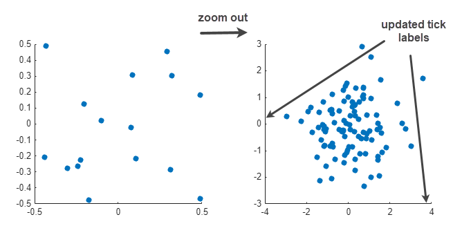
Two views of a scatter plot at different zoom levels. One view shows only a few scattered points within a small region. The other view is zoomed out and includes more points with updated ticks and tick labels.

Plots in Apps and MATLAB Online: Improved responsiveness when interacting with partially transparent 3-D plots

Interactions with partially transparent 3-D plots show improved responsiveness. To observe the improvement, the plot must be created in an app, in a figure created with the uifigure function, or in MATLAB Online.

For example, create a partially transparent surface plot of the peaks function evaluated over a 500-by-500 grid in an app window. Then drag to rotate the axes. On a Windows 11, Intel Xeon CPU W-2133 @ 3.60 GHz test system, the rotation is smoother and responds more quickly to the drag gesture in R2024a than in the previous release.

f = uifigure;
ax = axes(f);
Z = peaks(500);
surf(ax,Z,EdgeColor="none",FaceAlpha=0.4)
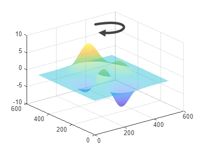
Rotation of a partially transparent surface plot

Software Development Tools

Project API: Find project files by label

You can now programmatically perform an advanced search in a project using the findFiles function. Supported workflows include:

  • Listing all files in a project

  • Filtering files that are not part of the project

  • Finding files by label or category name

  • Creating test suites from test files in a project and its references

Project API: Reanalyze all project dependencies

You can now programmatically reanalyze all files in your project and perform a complete dependency analysis by using the updateDependencies function.

Project API: Export list of project files to archive

You can now programmatically export a list of project files to an archive by using the export function.

For projects that have missing files, you can enable the export function to ignore the missing files.

Project Upgrade: Check for compatibility issues and upgrade project with improved usability and appearance

For projects that contain only MATLAB files, use Project Upgrade to check for compatibility issues with the current release. For projects that also contain Simulink models and libraries, you can apply fixes and automatically upgrade your project to the current release.

You can now easily interpret the upgrade results and examine the checks marked as need attention. You can also access frequent actions from the Project Upgrade toolstrip:

  • Rerun checks.

  • View changes that the upgrade applied.

  • Save results in a report.

For more information, see Check for Compatibility Issues Using Project Upgrade.

Project Upgrade tool with the toolstrip on top, list of files in the left pane, check details in the right pane, and results summary in the middle

Source Control: Support for signing Git commits

You can now enable the MATLAB Git integration to sign Git commits automatically. For more information, see Enable Signing Commits.

Source Control: Support for Git hooks

MATLAB Git integration can now run Git hooks with no additional setup. Starting in R2024a, you do not need to install Cygwin on Windows.

Supported hooks are pre-commit, commit-msg, post-commit, prepare-commit-msg, pre-push, pre-merge-commit, post-checkout, and post-merge. For more information, see Set Up Git Source Control.

Source Control API: Discard changes in Git repositories programmatically

You can now programmatically restore modified files in a Git repository using the discardChanges function.

Source Control in MATLAB Online: Expanded support for Git workflows

MATLAB Online now provides expanded support for Git workflows:

  • Squashing Git commits

  • Rebasing Git branches

Build Automation: Perform additional test and coverage analyses using TestTask class

You can produce additional test and coverage artifacts when using the matlab.buildtool.tasks.TestTask class:

  • Use the addCodeCoverage method to enable a task to collect code coverage information for your MATLAB source code. If you have a MATLAB Test™ license, you can also use the method to produce decision coverage, condition coverage, and modified condition/decision coverage (MC/DC) metrics.

  • If you have a Simulink Test license, you can export Simulink Test Manager results in MLDATX format by setting the TestResults property during task creation. If you also have a Simulink Coverage™ license, you can produce model coverage results by setting the ModelCoverageResults property during task creation or by using the addModelCoverage method.

Build Automation: Obfuscate source code using PcodeTask class

You can use the matlab.buildtool.tasks.PcodeTask class to create P-code files by obfuscating MATLAB source code as part of your build.

Build Automation: Build MEX file using MexTask class

You can use the matlab.buildtool.tasks.MexTask class to compile and link source files into a binary MEX file as part of your build.

Build Automation: Programmatically access code analysis results using CodeIssuesTask class

You can use the Results property of the matlab.buildtool.tasks.CodeIssuesTask class to programmatically access the results of code analysis. For example, you can return the paths to the code analysis results by using p = plan("check").Results.paths'. You can also specify the code analysis results as inputs of other tasks, for instance, plan("archive").Inputs = plan("check").Results.

Build Automation: Run tests in parallel

If you have a Parallel Computing Toolbox license, you can run tests in parallel by specifying the -parallel option of the buildtool command. This option affects only how matlab.buildtool.tasks.TestTask instances run. If you specify the -parallel option, the build runs the tests associated with TestTask instances in parallel.

Build Automation: Create initial build file

You can use the buildtool command to create a build file. To create a build file named buildfile.m in your current folder, execute buildtool -init. The resulting build file contains tasks created from built-in task classes in the matlab.buildtool.tasks namespace. You can use this build file as a starting point to define your build.

Build Automation: Disable incremental builds for task

You can disable incremental builds for a task. To force your task to rerun even if it is up to date, set the DisableIncremental property of the matlab.buildtool.Task instance to true.

Unit Testing Framework: Use renamed methods and name-value arguments when working with namespaces

MATLAB now refers to packages as namespaces. Some MATLAB unit testing methods and name-value arguments have been renamed to reflect this change. Their behavior remains the same.

This table shows the affected methods and their new names.

R2023b and EarlierStarting in R2024a
matlab.unittest.TestSuite.fromPackagematlab.unittest.TestSuite.fromNamespace
matlab.unittest.plugins.CodeCoveragePlugin.forPackagematlab.unittest.plugins.CodeCoveragePlugin.forNamespace

This table shows the affected name-value arguments and their new names. Use the IncludingInnerNamespaces name-value argument with the fromNamespace and forNamespace static methods, and use the IncludeInnerNamespaces name-value argument with the runtests, runperf, and testsuite functions.

R2023b and EarlierStarting in R2024a
IncludingSubpackages IncludingInnerNamespaces
IncludeSubpackages IncludeInnerNamespaces

There are no plans to remove support for existing references to the methods and name-value arguments.

Unit Testing Framework: Run tests using Test Browser in MATLAB Online

You can run script-based, function-based, and class-based tests using the Test Browser app in MATLAB Online.

Unit Testing Framework: Generate single-file HTML test report

You can generate a single-file HTML test report by using the matlab.unittest.plugins.TestReportPlugin.producingHTML or generateHTMLReport method. In a single-file HTML test report, all the contents of the report, such as text and images, are included in a single HTML file. In previous releases, these methods support only multifile test reports.

To generate a single-file HTML test report, specify the name of the test report file as an input to the method. For example, run your tests and generate an HTML test report contained in a single file named "myTestReport.html".

results = runtests("myTestFile.m");
generateHTMLReport(results,"myTestReport.html")

Unit Testing Framework: Control highlighting for covered or missed executables in interactive code coverage reports

You can control the highlighting of executables in an interactive code coverage report generated using either the matlab.unittest.plugins.codecoverage.CoverageReport class or the generateHTMLReport method. By default, the report highlights all the executables using different colors. To turn off highlighting for a group of executables, clear the corresponding check box in the Overall Coverage Summary section of the report. You can control the highlighting for covered, missed, or partially covered executables.

Unit Testing Framework: Modify HTML document title of code coverage report

You can modify the HTML document title when you generate a code coverage report using the matlab.unittest.plugins.codecoverage.CoverageReport class or the generateHTMLReport method. To modify the document title, specify the DocumentTitle name-value argument. For example, run your tests and generate a code coverage report with a specific HTML document title from the coverage results.

[testResults,coverageResults] = runtests("myTestFile.m", ...
    ReportCoverageFor=pwd)
generateHTMLReport(coverageResults,DocumentTitle="My Coverage Report")

Unit Testing Framework: Enable parallelizable plugins to work with default data if communication buffer is empty

The retrieveFrom method of the matlab.unittest.plugins.Parallelizable interface accepts a new input that lets you use default data if MATLAB workers cannot store the data that the plugin collects. For an example, see Extend Reporting of Finalized Test Suite Portion.

Unit Testing Framework: Use shared test fixtures in interactive tests

When you create an interactive test case from a test class using the matlab.unittest.TestCase.forInteractiveUse method, you can use the shared test fixtures associated with that test class for testing. For example, testCase = matlab.unittest.TestCase.forInteractiveUse(?MyTestClass,ApplySharedTestFixtures=true) sets up the shared test fixtures associated with MyTestClass when creating an interactive test case. The testing framework automatically tears down the shared test fixtures when the test case goes out of scope.

Unit Testing Framework: Respect element count when comparing sets

When you compare sets using the matlab.unittest.constraints.IsSameSetAs class, you can test whether elements occur the same number of times in the actual and expected sets. To respect the element count, set the RespectCount property of the constraint to true.

App Testing Framework: Perform scroll gestures on axes and UI axes

You can use the scroll method to test scroll gestures on axes and UI axes. Specify the direction of the scroll gesture to mimic a user scrolling up, down, left, or right.

App Testing Framework: Perform gestures on hyperlinks

You can use the press and chooseContextMenu methods to perform gestures on hyperlink components. For example, create a hyperlink and programmatically click it to open a URL.

fig = uifigure;
hlink = uihyperlink(fig);
hlink.Text = "MathWorks";
hlink.URL = "https://www.mathworks.com/";

testCase = matlab.uitest.TestCase.forInteractiveUse;
testCase.press(hlink)

 App Testing Framework: Node expanded callback executes when gestures programmatically expand tree nodes

To better mimic a user who must expand tree nodes to interact with a nested node, the node expanded callback executes when you perform a gesture on a collapsed tree node by using the choose or chooseContextMenu method. You can specify the callback by setting the NodeExpandedFcn property of the tree.

For example, perform a choose gesture on a nested node in a tree, and display the text of any programmatically expanded nodes.

fig = uifigure;
t = uitree(fig);
t.NodeExpandedFcn = @(src,event) disp(event.Node.Text);

parent = uitreenode(t,"Text","Runners");
child1 = uitreenode(parent,"Text","Joe");
child2 = uitreenode(parent,"Text","Linda");

testCase = matlab.uitest.TestCase.forInteractiveUse;
testCase.choose(child2)
 Compatibility Considerations

If you do not want the callback to execute, preserving the behavior in R2023b and earlier, expand the tree node before performing the gesture. In this code, the callback does not execute.

fig = uifigure;
t = uitree(fig);
t.NodeExpandedFcn = @(src,event) disp(event.Node.Text);

parent = uitreenode(t,"Text","Runners");
child1 = uitreenode(parent,"Text","Joe");
child2 = uitreenode(parent,"Text","Linda");

testCase = matlab.uitest.TestCase.forInteractiveUse;
expand(parent)
testCase.choose(child2)

 Functionality being removed or changed

Default build task name is empty string

Behavior change

By default, the Name property of the matlab.buildtool.Task class contains an empty string. In previous releases, the default value is a missing value.

Test Browser handles valid test files differently in the presence of invalid test files

Behavior change

The behavior of Test Browser has changed when a group of files includes both valid and invalid test files:

  • If you add tests to the test browser by selecting multiple test files, then the test browser imports the tests in the valid test files. In previous releases, the test browser does not import any tests if the group of selected files includes invalid test files.

  • If you run a group of both valid and invalid test files, then the test browser runs the tests in the valid test files. In previous releases, the test browser does not run any tests if the group includes invalid test files.

An invalid test file is a test file that the testing framework cannot run. Examples include a test file that contains syntax errors, a function-based test file that is missing local functions, and a file with a Test method that is passed an undefined parameterization property.

External Language Interfaces

 REST Function Service: Call user-defined MATLAB functions from any local or remote client program using REST

You can write client programs to call MATLAB using the MATLAB REST Function Service. The service uses HTTPS protocol, which enables communication between your programs and MATLAB regardless of your platform and execution environment. You can call custom MATLAB functions using any programming language or application that can make a REST call, either locally or remotely. For more information, see Call MATLAB Functions Using REST Function Service.

 Python Interface: Convert between MATLAB tables and Python Pandas DataFrames

You can now pass MATLAB tables or timetables directly to Python functions in MATLAB. MATLAB automatically converts the MATLAB table or timetable to a Python Pandas DataFrame.

Also, you can convert a Python Pandas DataFrame to a MATLAB table or timetable using the table or timetable function. For example, convert the Python Pandas DataFrame df to a MATLAB table and timetable.

T = table(df);
TT = timetable(df);

For more information, see Use Python Pandas DataFrames in MATLAB.

 Python Interface: Interactively run Python code with Run Python Live Editor Task

Use the Run Python Code task in the Live Editor to interactively run Python code or files and generate the corresponding MATLAB code. You can also use the Live Editor task to return Python variables in MATLAB, as well as pass MATLAB data to the Python code.

To add the task to a live script in the Live Editor, click Task on the Live Editor tab and select the Run Python Code icon.

For more information, see Run Python Code.

Python Interface: Convert between MATLAB and Python dictionaries

You can now pass MATLAB dictionaries directly to Python functions in MATLAB. MATLAB automatically converts the MATLAB dictionary to a Python dict. For example, pass a MATLAB dictionary d to the Python function print.

d = dictionary([10 20 30],[1 2 3]);
py.print(d)

Also, you can convert a Python dict to a MATLAB dictionary using the dictionary function.

pyDict = py.dict({{10,1},{20,2},{30,3}});
d = dictionary(pyDict);

For more information, see Use Python Dictionaries in MATLAB.

Publish C++ Interface: Share library definition file with publisher

You can share a MATLAB interface to a C++ library, for example by uploading the library definition files to GitHub. If other publishers have the same C++ library version and file structure as you do, then they can download the definition files and build the interface.

The files used to generate the interface, such as those specified by the InterfaceGenerationFiles argument of the clibgen.generateLibraryDefinition function, contain file specifications based on the folder structure of your computer. Starting in R2024a, you can specify file paths relative to an absolute path by specifying the RootPaths name-value argument as the beginning of the absolute path to the library files. Then another publisher can build the interface by updating the absolute path specified using the RootPaths dictionary based on the folder structure on their computer.

For an example, see Define Pathnames to Share Library Definition Files.

Publish C++ Interface: Use InterfaceName name-value argument, renamed from PackageName, to identify MATLAB interface to C++ library

MATLAB now refers to packages as namespaces. Some name-value arguments and properties used to publish a MATLAB interface to a C++ library have been renamed to reflect this change. Their behavior remains the same.

  • In the clibgen.generateLibraryDefinition function, the PackageName name-value argument is now named InterfaceName.

  • In the clibgen.buildInterface function, the PackageName name-value argument is now named InterfaceName.

  • In the clibgen.LibraryDefinition class, the PackageName property is now named InterfaceName.

Use InterfaceName to identify the MATLAB interface to a specific C++ library. For example, if you set InterfaceName to "libname", then function calls to the library have this format:

retVal = clib.libname.funcname(arg1,arg2,...)

There are no plans to remove support for existing references to the arguments and property.

Call C++ from MATLAB: Use string for C++ enum parameter

You can pass a MATLAB string to a C++ function or method in C++ library libname that accepts clib.libname.enum as an input argument. For more information, see the string scalar entry in the MATLAB Type to C++ Type Mapping table.

Call MATLAB from C++: Support for data types in matlab::engine::MATLABEngine functions feval and fevalAsync

The matlab::engine::MATLABEngine member functions feval and fevalAsync support native C++ string, std::vector, and std::complex data types. For more information, see the RhsArgs&&... rhsArgs entry in the feval and fevalAsync Parameters tables.

Call MATLAB from C++: Support for handle classes in strongly typed C++ interface

You can include handle classes in a strongly typed C++ interface when you call the matlab.engine.typedinterface.generateCPP function. The function creates code with handle copy behavior. That is, functions and methods can modify the input data in the calling workspace without making copies. For more information, see Use MATLAB Handle Classes in C++.

The function does not generate code to support dynamic properties, the set and get behavior for graphics handles, listener workflows, or the findprop, findobj, and delete handle methods.

Call MATLAB from C++: Support for comparison operators

The matlab.engine.typedinterface.generateCPP function generates C++ comparison methods and the isvalid function as well as comparison operators for both handle and value classes, which implement the eq, ne, lt, gt, le, and ge methods in MATLAB.

Code generated for comparison operators like == have a Boolean output type. If you override the eq function in MATLAB with a non-Boolean output, then you must use the eq method in your application instead of ==.

Call MATLAB from C++: Use Namespaces name-value argument, renamed from Packages, with matlab.engine.typedinterface.generateCPP function

In the matlab.engine.typedinterface.generateCPP function, the Packages name-value argument is now named Namespaces. The behavior of this name-value argument remains the same. There are no plans to remove support for existing references to the argument.

Java: MATLAB support for OpenJDK™ 17

As of R2024a, MATLAB supports OpenJDK 17 from https://adoptium.net/. For supported version information, see MATLAB Interfaces to Other Languages.

 .NET Interface: Support for .NET 6

On Microsoft Windows platforms, MATLAB supports .NET 6 and higher, in addition to existing support for the Microsoft .NET Framework. To select a .NET environment, use the dotnetenv function. For more information, see Selecting .NET Core in MATLAB.

 Compatibility Considerations

For more information about changes to .NET support, see .NET Interface: .NET 5 is no longer supported.

Call MATLAB from .NET: Support for dictionary objects

You can convert a .NET object whose type implements the System.Collections.Generic.IDictionary<TKey,TValue> interface to a MATLAB dictionary.

You can convert a MATLAB dictionary to any of these .NET types:

  • System.Collections.Generic.Dictionary<TKey,TValue>

  • System.Collections.Generic.IDictionary<TKey,TValue>

  • System.Collections.Generic.IReadOnlyDictionary<TKey,TValue>

  • System.Collections.IDictionary

For more information, see:

For examples, see Use MATLAB Dictionary Objects in .NET.

Call MATLAB from .NET: Support for handle classes in strongly typed C# interface

You can include handle classes in a strongly typed C# interface when you call the matlab.engine.typedinterface.generateCSharp function. The function creates code with handle copy behavior. That is, functions and methods can modify the input data in the calling workspace without making copies.

The function does not generate code to support dynamic properties, the set and get behavior for graphics handles, listener workflows, or the findprop and findobj handle methods. For more information, see Use MATLAB Handle Classes in C#.

Call MATLAB from .NET: Support for comparison operators

The matlab.engine.typedinterface.generateCSharp function generates C# comparison methods and the isvalid function as well as comparison operators for both handle and value classes, which implement the eq, ne, lt, gt, le, and ge methods in MATLAB.

Code generated for comparison operators like == have a Boolean output type. If you override the eq function in MATLAB with a non-Boolean output, then you must use the eq method in your application instead of ==.

Call MATLAB from .NET: Support for IConvertible interface

You can use the .NET IConvertible interface to convert the value of a reference or value type to a common language runtime type with an equivalent value.

C# Code (R2023b and earlier)

C# Code (Since R2024a)

MATLABArray retval = matlab.eval("int32(42)");
dynamic retvalDynamic = retval;
double d = retvalDynamic;
MATLABArray retval = matlab.eval("int32(42)");
double d = Convert.ToDouble(retval);

Widening conversion occurs when a value of one type is converted to another type that is of equal or greater size. The .NET type does not need to exactly match the MATLAB type, if the conversion is lossless.

double d = matlab.eval("int32(42)");
float f = matlab.eval("uint8(42)");

For conversion information, see MATLAB Numeric Types in .NET.

Call MATLAB from .NET: Use Namespaces name-value argument, renamed from Packages, with matlab.engine.typedinterface.generateCSharp function

In the matlab.engine.typedinterface.generateCSharp function, the Packages name-value argument is now named Namespaces. The behavior of this name-value argument remains the same. There are no plans to remove support for existing references to the argument.

Compilers: Support for MinGW64 Compiler (Fortran)

MATLAB supports the MinGW64 Compiler (Fortran) for building Fortran MEX files and standalone MATLAB engine and MAT-file applications on Windows platforms. For installation instructions, see MATLAB Support for MinGW-w64 C/C++/Fortran Compiler. For an up-to-date list of supported compilers, see Supported and Compatible Compilers.

 Functionality being removed or changed

Ctrl+C stops execution of webread, webwrite, websave, and functions in the HTTP interface

Behavior change

Pressing Ctrl+C while executing the MATLAB functions webread, webwrite, and websave, as well as functions in the MATLAB HTTP interface, stops execution of the MATLAB command. This behavior is consistent with how other MATLAB functionality handles Ctrl+C, as described in Use Keyboard Shortcuts to Navigate MATLAB. Previously, the functions threw a custom exception that you could catch inside a try/catch block. If your code contains try/catch blocks, you can update your code by removing them. For an example, see Ctrl+C stops execution of MATLAB command in the matlab.net.http.Disposition class.

Additionally, the matlab.net.http.Disposition enumeration class no longer supports the Interrupt enumeration member. Previously, matlab.net.http.Disposition.Interrupt created a matlab.net.http.LogRecord object if you interrupted a command by pressing Ctrl+C.

load function no longer restores COM object from MAT-file

Behavior change

If you save a COM object from the workspace to a file using the save function, you can no longer reload it into the workspace as a COM object using the load function. Starting in R2024a, the load function displays a warning when trying to load COM objects and loads the data using another data type.

Previously, load attempted to load COM objects, but the restored data was limited. For example, if you saved an instance of a Microsoft Excel® COM server to a file, MATLAB saved the Excel session, but did not save any objects created in the session. If you tried to load the object into the workspace, load did not fully restore the original COM object.

.NET Interface: .NET 5 is no longer supported

Errors

Support for .NET 5 is discontinued. For continued support for your applications, upgrade to a supported version of .NET. For information about .NET versions compatible with MATLAB, see MATLAB Interfaces to Other Languages.

Perl 5.38.2: MATLAB support on Windows

Behavior change

As of R2024a, MATLAB on Windows ships with an updated version of Perl, version 5.38.2.

If you use the perl command on Windows platforms, see https://www.perl.org/ for information about using this version of the Perl programming language. For a standard distribution of HTML::Parser, source code, and information about using HTML::Parser, see https://metacpan.org/pod/HTML::Parser.

Hardware Support

Hardware Boards, Cameras, and Drones: Documentation for hardware support packages moved to MATLAB documentation

Starting in R2024a, the documentation for these support packages is included in the MATLAB documentation and all updates will be announced in the MATLAB release notes:

  • MATLAB Support Package for Arduino Hardware

  • Raspberry Pi Blockset

  • MATLAB Support Package for BeagleBone® Black Hardware

  • MATLAB Support Package for LEGO® MINDSTORMS® EV3 Hardware

  • MATLAB Support Package for USB Webcams

  • MATLAB Support Package for IP Cameras

  • MATLAB Support Package for Parrot® Drones

  • MATLAB Support Package for Ryze Tello Drones

In previous releases, the support package documentation was installed when you installed the support package software. To access archived release notes from the previous release, use these links:

Arduino Hardware: Support on macOS with Apple silicon

You can now use MATLAB Support Package for Arduino Hardware on macOS with an Apple silicon processor in the installed version of MATLAB.

Arduino Hardware: Read data from ADIS16505 sensor

MATLAB Support Package for Arduino Hardware enables you to read linear acceleration and angular velocity along the x-, y-, and z- axes as well as temperature from the ADIS16505 sensor connected to the SPI bus of an Arduino board. Use the new adis16505 object and associated functions to create a connection to the ADIS16505 sensor and read values.

Arduino Compatible Boards: ESP32 core version update

MATLAB Support Package for Arduino Hardware now supports ESP32 core version 2.0.11. The updated core is installed when you install the support package.

Raspberry Pi Hardware: Support for Debian Bullseye with kernel 6.1.21 and above

Raspberry Pi Blockset now supports Debian Bullseye with kernel 6.1.21 and above. This support is available when you use the support package in the installed version of MATLAB or in MATLAB Online.

Raspberry Pi Hardware: Support on macOS with Apple silicon

You can now use Raspberry Pi Blockset on macOS with an Apple silicon processor. This support is available when you use the support package in the installed version of MATLAB or in MATLAB Online.

USB Webcams: Retrieve property metadata for webcam object using propertyInfo function

You can use the propertyInfo function of a webcam object to retrieve metadata, such as Name, Type, Default, ReadOnly, and AllowedValues, for all the properties supported by your webcam.

USB Webcams: Use webcam objects as dictionary keys and values

Starting in R2024a, you can use webcam objects as keys or values in a dictionary. You can also perform basic dictionary operations on webcam objects using related functions. For more information, see Dictionaries.

 Functionality being removed or changed

Raspberry Pi Hardware: Support for Stretch operating system has been removed

Errors

Starting in R2024a, you can no longer use Raspberry Pi Blockset to communicate with Raspberry Pi hardware that uses the Raspbian Stretch operating system.

R2023b

New Features, Bug Fixes, Compatibility Considerations

Environment

 Live Editor Tasks: Create Live Editor task from selected code with interactive controls

You can convert a selection in the Live Editor that contains code, text, and interactive controls into your own Live Editor task. Supported controls include numeric sliders, numeric spinners, drop-down lists, check boxes, edit fields, buttons, and file browsers.

To create your own Live Editor task from a selection, after making the selection, go to the Live Editor tab, and in the Code section, select Task > Convert to Task. When prompted, enter a name for the task, the name of the task class definition file to create, an optional description of the task, and some optional keywords. MATLAB creates your Live Editor task from the selection and adds the task to the Live Editor task gallery.

To add your task to a live script, on the Live Editor tab, click Task and select your task from the list.

For more information, see Create Live Editor Task from Selection.

 Live Editor Tables: Add tables containing text and images to live scripts and functions

You can add tables to your live scripts and functions to format text and images. To insert a table, go to the Insert tab and select Table drop-down arrow. Move the cursor over the grid to highlight the numbers of rows and columns you want and then click to add the table. To create a larger table, select the Insert a table button and specify the numbers of rows and columns in the dialog box.

After inserting the table, to modify its rows and columns, right-click the table, select Table, and select from the available options. For more information, see Format Text in the Live Editor.
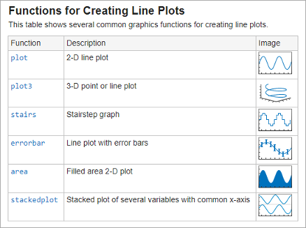
Live script with a table containing three columns, a header row, and six additional rows. The table contains text, hyperlinks, and images.

 Live Editor Controls: Add color pickers and state buttons to live scripts

You can add a color picker to your live script to select a color interactively. You also can add a state button to indicate and interactively set the value of a logical variable.

To add a color picker, go to the Live Editor tab, and in the Code section, select Control > Color Picker. To add a state button, select State Button.
Color picker with the color blue selected, assigned to the variable color. State button in the selected state, assigned to the variable lightsOn.

For more information, see Add Interactive Controls to a Live Script.

Live Editor Controls: Select folders interactively in live scripts using file browser

You can use a file browser in a live script to select a folder interactively. To add a file browser, go to the Live Editor tab, and in the Code section, select Control > File Browser. To configure the control to select a folder rather than a file, right-click the control and select Configure Control. Then, in the Type section, select Folder.

For more information, see Add Interactive Controls to a Live Script.

Live Editor Accessibility: Interact with inline output using the keyboard

You can now use keyboard shortcuts to interact with inline output in live scripts. To move focus from the code to the output, use the down arrow and up arrow keys. To activate an output, press Enter. Once an output is activated, you can scroll text using the arrow keys, navigate through hyperlinks and buttons using the Tab key, and open the context menu by pressing Shift+F10. To deactivate an output, press Esc.

To disable using the keyboard to move focus to the output when output is inline, on the Home tab, in the Environment section, click Preferences. Select MATLAB > Editor/Debugger > Display, and clear the Focus outputs using keyboard when output is inline option.

Live Editor Export: Interactively customize export options, such as document paper size, orientation, margins, and figure format

When exporting to PDF, Microsoft Word documents, HTML, and LaTeX, you can use the Export dialog box to customize export options interactively. To open the Export dialog box, on the Live Editor tab, click Export and then select an export format. In MATLAB Online, click Save instead of Export.

You can change the paper size, orientation, and margins when exporting to PDF, Microsoft Word documents, and LaTeX. You also can change the resolution and format of figures when exporting to PDF, HTML, and LaTeX (requires the files to be run before exporting).
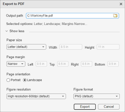
Export to PDF dialog box, with an edit field for specifying the output path, and several drop-down lists and radio buttons for specifying paper size, page margin, page orientation, figure resolution, and figure format

For more information, see Ways to Share and Export Live Scripts and Functions.

 export Function: Convert live scripts and functions to Markdown files and Jupyter notebooks

You can convert live scripts and functions to Markdown files and Jupyter notebooks by using the export function. To convert a live script or function to a Markdown file or Jupyter notebook, specify an output filename with a .md or .ipynb extension. Alternatively, you can set the Format name-value argument to "Markdown" or "ipynb".

For example, convert the live script "penny.mlx" to a Markdown file and a Jupyter notebook.

export("penny.mlx","penny.md")
export("penny.mlx","penny.ipynb")

Editor Execution: Run sections even if other sections contain syntax errors

In the Editor and Live Editor, you can now run a code section even if another section in the file contains a syntax error. Previously, you could run a section only if the entire file contained no syntax errors.

For more information about creating sections, see Create and Run Sections in Code.

Editor Variable Renaming: Automatically rename next references to variables or functions in file

In the Editor and Live Editor, when you rename a variable or function in a file, you can choose whether to rename all instances or only the instances from the current cursor location to the end of the file. To rename all instances of a variable or function, press Shift+Enter. To rename only the instances from the current cursor location to the end of the file, press Alt+Shift+Enter. On macOS, use Option+Shift+Enter instead.

For more information, see Find and Replace Text in Files and Go to Location.

Find and Replace Dialog Box: Use capture groups in regular expressions to search for and replace groups of characters

Search for and replace groups of characters in a file using capture groups in regular expressions. To begin searching using regular expressions, on the Editor or Live Editor tab, in the Navigate section, click Find. Then, select the Regular expression option .

To create a capture group, surround the characters that you want to group with parentheses. Then, to access the capture group within the regular expression, use the format \number, where number refers to the capture group number. To access the capture group within a replacement pattern, use the format $number. For example, to find duplicate words in a file, use the expression (\w+)\s\1. To replace the two words with just one word, use the expression $1.

Find and replace dialog box with a regular expression containing a capture group in the Find and Replace fields

You also can create a named capture group using the format ?<name>, where name is the name of the capture group. Then, to access the named capture group, use the format \k<name> within the regular expression, or $<name> within a replacement pattern. For example, to find duplicate words using a named capture group, use the expression (?<myword>\w+)\s\k<myword>. To replace the two words with just one word, use the expression $<myword>.

Find and replace dialog box with a regular expression containing a named capture group in the Find and Replace fields

For more information about searching using the find and replace dialog box, see Find and Replace Text in Files and Go to Location.

Debugging in MATLAB Online: Manage breakpoints and navigate the function call stack using Debugger panel

Use the Debugger panel to manage breakpoints and navigate the function call stack while debugging in MATLAB Online. To open the Debugger panel, go to the Editor or Live Editor tab, and in the Analyze section, click Debugger. You also can open the panel using the Open more panels button (three-dot icon) in the sidebar.

Debugger panel showing a breakpoints section and a function call stack section. The breakpoints section shows Pause on Errors enabled, as well as three enabled breakpoints in a code file

For more information, see Debug MATLAB Code Files.

Desktop Layout in MATLAB Online: Open additional panels directly from sidebars

In MATLAB Online, you can open additional panels (also referred to as tools) directly from the sidebars. To open additional panels, in a sidebar, click the Open more panels button (three-dot icon). Then, in the Open Panel dialog box, select from the available panels. You also can right-click in a sidebar and select Open more panels.

For example, to open the Code Issues panel, click the Open more panels button (three-dot icon), and select the Code Issues panel.

MATLAB Online desktop with the Open more panels buttons circled in the left and bottom sidebars. The Open Panel dialog box shows the available panels: Code Issues, Command History, Command Window, Debugger, Files, Find Files, Source Control, and Workspace.

For more information, see Change Desktop Layout.

Themes in MATLAB Online: Save color customizations for individual themes

MATLAB Online now saves your color customizations for each available theme. If you customize the colors of the MATLAB Online desktop and then the MATLAB theme changes to a new theme or to match a change to the operating system color scheme, your customizations are saved.

With this change, in MATLAB Online, programmatically customizing syntax highlighting colors using the matlab.colors settings is no longer supported. To customize syntax highlighting colors, use the preferences in the MATLAB Appearance Colors Preferences page of the Preferences window instead. For more information, see Change Desktop Colors.

In an installed version of MATLAB, programmatically customizing syntax highlighting colors using the matlab.colors settings is still supported.

Window Management in MATLAB Online: Automatically collapse windows

In MATLAB Online, when you click the MATLAB background, open windows in the foreground collapse. Collapsing a window reduces the size of the window by displaying only its title bar.

Title bar with title and buttons

To restore the collapsed windows, click the title bar of one of the previously open windows. To prevent a window from being collapsed or minimized, click Pin on its title bar.

For more information, see Manage Windows in MATLAB Online.

 MATLAB on Macs: Better performance and improved battery life on MacBooks with MATLAB and Simulink running natively on Apple silicon

You can run MATLAB and Simulink natively on MacBook computers with Apple silicon.

MATLAB on Macs: Java Runtime Environment required for MATLAB and MATLAB Runtime on Apple silicon

On Mac computers with Apple silicon, if MATLAB or MATLAB Runtime does not find a supported Java Runtime Environment (JRE), the program displays a dialog box with a link to information about the Java requirement and the recommended solution. For information about the recommended solution, see https://www.mathworks.com/support/requirements/apple-silicon.html. For more information, see Start MATLAB on macOS Platforms.

MATLAB Drive: New URL for MATLAB Drive Online (January 2024)

You can now access MATLAB Drive Online at https://drive.mathworks.com. Previously, MATLAB Drive Online was located at https://drive.matlab.com.

 Functionality being removed or changed

MATLAB Online keyboard shortcuts Ctrl+0, Ctrl+1, Ctrl+2, and Ctrl+3 have been removed

The Ctrl+0, Ctrl+1, Ctrl+2, and Ctrl+3 keyboard shortcuts have been removed in MATLAB Online to avoid a conflict with the shortcuts to switch tabs in certain browsers. These shortcuts were previously used to make the Command Window, Command History, Files panel, or Workspace panel active. On macOS, the corresponding keyboard shortcuts (Command+0, Command+1, Command+2, and Command+3) have also been removed.

To make one of these tools active, use Ctrl+F6 and Ctrl+Shift+F6 to move forward or backward through the different areas of the MATLAB Online desktop until your intended tool is selected. Then, to navigate into the tool, press the Tab key. On macOS, use the Command key instead of the Ctrl key.

XML comparison type for visdiff function will be removed

Warns

The XML comparison type for the visdiff function will be removed in a future release. Overriding the default comparison type by specifying "xml" will not be supported in a future release. In R2023b, scripts that use visdiff(filename1,filename2,"xml") issue a warning.

Language and Programming

configureDictionary Function: Create dictionaries with configured keys and values

Use the configureDictionary function to create an empty dictionary with specified types for keys and values.

For example, create a dictionary that is configured to accept strings as keys and doubles as values.

d = configureDictionary("string","double")
d =

  dictionary (string ⟼ double) with no entries.

lookup, insert, and remove Functions: Find, add, and remove dictionary entries

You can perform basic dictionary operations using these three new functions:

• lookup — Find the value that corresponds to a key. You can optionally specify a fallback value for the function to return if it cannot find the entry.

• insert — Add new dictionary entries. You can optionally specify whether to overwrite existing entries.

• remove — Remove dictionary entries.

codeIssues Object: Export issues identified in code

Use the export object function of the codeIssues object to write its issues to a file. Exported files are in SARIF format by default, but you can specify to export issues in SonarQube or MATLAB encoded JSON formats.

Code Compatibility Analyzer App: Group and filter code issues with improved interface

The Code Compatibility Analyzer app has a new interface that makes it easier to navigate issues found in code. You can now adjust how identified issues are grouped and filter results by text, severity, and issue type.
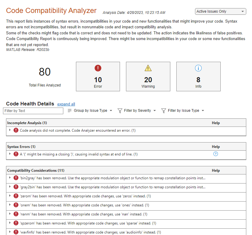
Code Compatibility Analyzer interface from R2023b, with a summary of code issues at the top and a grouped and filtered list of issues at the bottom

Class Diagram Viewer: Add known subclasses to diagrams

You can now automatically add one or more layers of known subclasses of a class in a diagram. Right-click the class in a diagram to see the options for adding subclasses. See Class Diagram Viewer for more information.

mustBeSparse Function: Validate sparsity of arguments

Use the mustBeSparse validation function to check whether an argument is sparse. This function is designed for use in function argument validation and property validation.

MATLAB backgroundPool Function: load function supported in background threads

Use the load function in thread-based environments, including the MATLAB backgroundPool. Saving Version 7.3 MAT-files is not supported.

 Functionality being removed or changed

Arrays contained in structure fields, cells, and class properties are displayed with partial contents as well as size and data type

Behavior change

Between R2021b and R2023b, MATLAB displayed the entire contents of an array in a structure field, cell, or class property if the contents fit in the display. If the array did not fit, MATLAB showed as much of the array as the display allowed.

Starting in R2023b, if the entire contents of an array in a structure field, cell, or class property do not fit in the display, MATLAB shows as much of the array as the display allows, as well as the size and data type of the array. For example, as of R2023b, MATLAB displays partial contents as well as size and data type for a cell that contains an array of 100 double values.

D = {3.14,[1:100]};
D(2)
ans =

  1×1 cell array

    {[1 2 3 4 5 6 7 8 9 10 11 12 13 14 15 16 17 18 … ] (1×100 double)}

The disp function follows the same behavior for structures, cells, and class properties.

For more information, see the Version History notes in cell and struct.

Using the AbortSet attribute and a get method that sets the property value can cause infinite recursion

Behavior change

Generally, MATLAB calls a property set method, if one exists, when a property is set outside of the set method. When a property has a set method and uses the AbortSet attribute, MATLAB acquires the old value and compares it with the new value for any assignment to that property outside of its set method. If the property has a get method, the get method is called to acquire the old value.

For R2023b, the get method is no longer bypassed when it indirectly results in another call to the get method because of the AbortSet check. This removes overhead from many property access operations. As a result, MATLAB calls the get method again to acquire the old property value when a property fits all three of these conditions:

  • The property uses the AbortSet attribute.

  • The property has a set method.

  • The property has a get method that assigns a value to the property.

This call to get could lead to infinite recursion if the property assignment in the get method is unconditional.

Malformed and reserved import arguments issue warning

Behavior change

Previously, the import function accepted malformed arguments, such as #.b or a.*.*, and MATLAB still executed the command even though nothing was imported. It also allowed importing of reserved names, such as a.for or a.if that do not satisfy MATLAB naming rules. Starting in R2023b, MATLAB issues a warning if you include invalid imports. Such imports will not be supported in a future release.

ver and verlessthan are not recommended

Still runs

Using ver to return the current MATLAB release information is not recommended. Use matlabRelease instead.

Using verlessthan to determine if the current MATLAB release is older than a specified release is not recommended. Use isMATLABReleaseOlderThan instead.

Change to precedence for constructors in class folders

Behavior change in future release

When a class and a function on the path have the same name, MATLAB currently gives precedence to the class constructor if the class is defined inside a class folder (@-folder). The constructor takes precedence even if the function appears before the class on the path.

In a future release, this precedence rule will be removed. In other words, if a function appears before a class of the same name on the path, the function will have precedence regardless of whether the class is defined in a class folder. Change the order of these items on your path to maintain your preferred precedence.

Defining classes and packages: Using schema.m will not be supported in a future release

Still runs

Support for classes and packages defined using schema.m files will be removed in a future release. Replace existing schema-based classes with classes defined using the classdef keyword.

Data Analysis

 Experiment Manager App: Design experiments to run MATLAB code, and visualize, filter, and compare results

Create an experiment to run your MATLAB code using a range of parameter values and compare the results by using the Experiment Manager app. For example, you can use an experiment to explore how the solution to a system of differential equations responds to different coefficient values or how it evolves from different initial conditions. When you run the experiment, Experiment Manager runs your code in multiple trials, each one using a different combination of parameter values.

Experiment Manager provides visualizations, filters, and annotations to help you manage your experiment results and record your observations. To improve reproducibility, Experiment Manager stores a copy of the experiment definition every time that you run an experiment. You can access past experiment definitions to keep track of the parameter values and MATLAB code that produce each of your results.

By default, Experiment Manager runs one trial at a time. If you have Parallel Computing Toolbox, you can run multiple trials at the same time or run a single trial at a time on multiple GPUs, on a cluster, or in the cloud. If you have MATLAB Parallel Server™, you can also offload experiments as batch jobs in a remote cluster so that you can continue working or close your MATLAB session while your experiment is running.

If you have Deep Learning Toolbox or Statistics and Machine Learning Toolbox, you can use Experiment Manager for your AI workflows. For more information, see Experiment Manager (Deep Learning Toolbox) or Experiment Manager (Statistics and Machine Learning Toolbox).

 Pivot Table Live Editor Task: Interactively summarize tabular data in pivoted table

Use the Pivot Table task in the Live Editor to interactively perform a pivoting operation on data in a table or timetable. You can filter the input table, specify grouping variables to designate pivoted table rows and columns, customize the format and contents of the pivoted table, and visualize the pivoted table in a chart. To add the task to a live script in the Live Editor, click Task on the Live Editor tab and select the Pivot Table icon.

resize, paddata, and trimdata Functions: Change the size of data by adding or removing elements

Change the size of array or tabular data by using the resize, paddata, and trimdata functions. You can specify the dimensions to operate along, the fill value or pattern for padding, and the side of the input data for resizing.

  • resize adds or removes elements depending on if the length of the input data is less than or greater than the target length. The resized data matches the target length.

  • paddata only adds elements. If the length of the input data is greater than or equal to the target length, the output data is the same as the input data.

  • trimdata only removes elements. If the length of the input data is less than or equal to the target length, the output data is the same as the input data.

smoothdata2 Function: Smooth noisy data in two dimensions

Smooth noisy entries in two-dimensional data sets with a moving window method by using the smoothdata2 function. You can customize the smoothing method and moving window size, specify how missing values are handled, adjust the level of smoothing, and specify the sample points used by the smoothing method.

kde Function: Estimate a probability function by using kernel density estimation for univariate data

Estimate a probability function with kernel density estimation for univariate data by using the kde function. Optionally define parameters such as the probability function to estimate, points at which to evaluate the estimated probability function, and type of kernel smoothing function.

Join Tables Live Editor Task: Sort output timetable by row times when row times are not key values

When the left input of the Join Tables task in the Live Editor is a timetable, you can sort the output timetable by row times even when you do not specify row times as key values. To sort by row times in this case, select the Sort result by row times check box. In previous releases, Join Tables does not provide this sorting option.

This sorting option is available only when all three of these conditions are true:

  • The left input is a timetable that is sorted by row times.

  • You specify an outer join or an inner join.

  • You do not specify row times as key values.

In all releases, the output timetable is automatically sorted by row times when you specify that row times are key values.

Data Cleaning: Interactively fill missing data with values from nearest neighbor rows

Fill missing entries with the mean of nearby points by using the K-nearest neighbors fill method in the Clean Missing Data task in the Live Editor or the Clean Missing Data cleaning method in the Data Cleaner app. Specify the number of neighbors, and define the distance between rows using the Euclidean distance, the scaled Euclidean distance, or in the Clean Missing Data task, a custom function.

Live Editor: Display the contents of nested tables as variables

Starting in R2023b, the output of the Live Editor displays the contents of tables or timetables that contain nested tables or timetables as variables inline. You can interactively manipulate a nested table, for example, by selecting or sorting a variable or copying a variable with its headers. Previously, the output of the Live Editor displayed the dimensions of nested tables, but not the nested table contents.

For example, use the Pivot Table task to create nested tables. The Live Editor output displays the complete pivoted table contents.
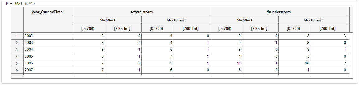
Live Editor output of a table with variables containing three levels of nesting. The output displays the contents of the nested tables.

Live Editor: Copy output data as tab-delimited text

You can copy data from the output of the Live Editor as tab-delimited text. Select some data in the output, and copy the data by pressing Ctrl+C or by right-clicking the data and selecting Copy Selection. Then, paste the tab-delimited text. The pasted text respects the rows and columns from the Live Editor output. For example, select and copy the elements in a row vector, and paste the selection into a Microsoft Excel worksheet. The first element of each worksheet column contains an element from the copied vector.

pivot Function: Display empty groups in pivoted table

Include, rather than omit, empty groups in the pivoted table returned by the pivot function by setting the IncludeEmptyGroups name-value argument to true. An empty group occurs when a possible value of a variable specified by Columns or Rows is not represented in the input table, such as in a categorical, logical, or binned numeric variable.

pivot Function: Specify row names for pivoted table as row group names

In a pivoted table returned by the pivot function, you can now place row labels to the left of the leftmost table variable by setting the RowLabelPlacement name-value argument to "rownames". This option sets the RowNames property of the pivoted table to the row group names. If Rows specifies multiple variables, the row labels are the group names concatenated with an underscore. Previously, the pivoted table always placed row labels in the leftmost table variables.

stackedplot Function: Plot events associated with timetables

The stackedplot function can plot events as lines or shaded regions on stacked plots created from timetables. To plot events associated with a timetable, you must attach an event table to it before you call stackedplot. For more information on event tables, see eventtable.

To support events, stackedplot has a new EventsVisible name-value argument:

  • If EventsVisible is "on", then stackedplot plots events as lines or shaded regions.

  • If EventsVisible is "off", then stackedplot hides events.

Stacked plot of timetable data with events plotted as shaded regions

Timetable Events: Perform calculations directly on event tables without extracting their data

You can now perform calculations directly on event tables without extracting their data. In R2023a, you cannot perform direct calculations on event tables, though you can perform direct calculations on tables and timetables.

For more information, see Direct Calculations on Tables and Timetables and Rules for Table and Timetable Mathematics.

containsrange, overlapsrange, and withinrange Functions: Specify time ranges by using event filters

You can specify a time range by using event filters when you use the containsrange, overlapsrange, or withinrange function. To use event filters, you must first attach an event table to the input timetable. For more information on using these functions with event filters, see eventfilter.

Variables Editor in MATLAB Online: Interactively change display format for datetime or duration data

In the Variables editor in MATLAB Online, you can interactively modify the display format for datetime or duration variables. Right-click the variable or column header, select Modify Date/Time Format, and choose from the list of display formats or specify a custom display format. The Command Window displays the corresponding code. Previously, interactively changing the display format for datetime data was supported only in the installed version of MATLAB. Interactively changing the display format for duration data was not supported.

Variables Editor in MATLAB Online: View and interactively edit scalar structures, object arrays, and tables with grouped variables

The Variables editor in MATLAB Online has improved functionality for these data types:

  • Scalar structure — You can now view, expand, and interactively edit the fields and nested fields in a scalar structure. Previously, you had to open each field in another tab in the Variables editor to view and edit its contents.
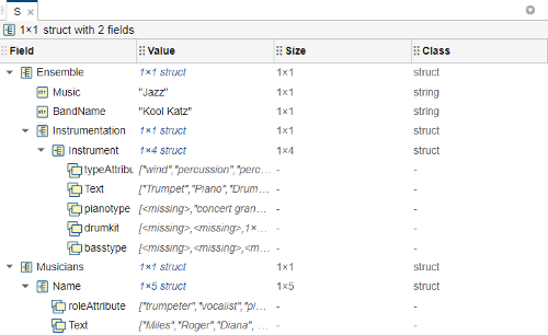
    Scalar structure with fields and nested fields expanded in the Variables editor. The triangle icons expand and collapse the fields.

  • Object array — You can now view and interactively edit the values of common properties of objects in an object array. Previously, you had to open each object in a separate tab in the Variables editor to view and edit its property values.
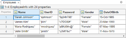
    Object array of four objects in the Variables editor. The common properties are variables in the table display. The objects are rows in the table display. The current selection is the value of a property for an object in the array.

  • Table with grouped variables — You can now select and interactively edit the contents of a subcolumn in a group of table variables. Previously, interactively editing a subcolumn in a group of table variables was not supported.
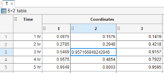
    Table that contains three grouped variables in the Variables editor. The three grouped variables appear as three subcolumns. The current selection is one cell of a subcolumn.

Accessibility in MATLAB Online: Use a screen reader to interact with the Workspace browser, Variables editor, Property Inspector, and Import Tool

In MATLAB Online, when using a screen reader, you hear additional information about these interactions:

  • When you add variables to or remove variables from the MATLAB workspace, you hear the number of variables added or removed.

  • When you open a variable in the Variables editor, you hear the summary of the variable.

  • When you edit a graphics object property using a drop-down list in the Property Inspector, you hear the value. Previously, all Property Inspector components had screen reader support except for drop-down list items.

  • When you successfully import a variable using the Import Tool, you hear the success message after the import is complete.

Histogram Distribution Charts: Calculate values and create histograms using percentages

You can create histograms with percentages on the vertical axis by using the histogram and histogram2 functions. You can normalize histogram values as percentages by using the histcounts and histcounts2 functions. For each function, set the Normalization name-value argument to "percentage".

tallrng Function: Specify random number algorithm without specifying seed

When using the tallrng function, you can specify just the algorithm for the random number generator to use. The tallrng(generator) syntax allows you to set the random number algorithm without specifying the seed, where tallrng uses a seed of 0. This syntax is equivalent to tallrng(0,generator). For example, tallrng("philox") initializes the Philox 4x32 generator with a seed of 0.

 Functionality being removed or changed

min and max functions will no longer support specifying second input array as character array

Warns

For the min and max functions, specifying a second input array as a character array issues a warning and will not be supported in a future release. This change minimizes confusion with options that can be specified as character vectors, such as the missing value condition. To maintain the previous functionality, you can convert the second input array to double, for example, max(A,double(B),'includenan').

Data Import and Export

readstruct Function: Read data from JSON files

Read data from JSON files into MATLAB structure arrays using the readstruct function. For example, S = readstruct("myFile.json") creates a structure S from myFile.json.

writestruct Function: Write structure arrays to JSON files

Write MATLAB structure arrays to JSON files using the writestruct function. For example, writestruct(S,"myFile.json") writes the data in structure S to myFile.json.

Parquet: Create ParquetDatastore objects more efficiently with partition control in parallel environments

In parallel environments, you can create a ParquetDatastore object more efficiently by specifying the unit of partition and the size of partition blocks. Specify the new PartitionMethod and Blocksize name-value arguments during creation of the datastore.

cmdsep Function: Return command separator for current platform

Return the platform-specific command separator character using the cmdsep function. You can create a chain of commands by using cmdsep with system. For example, system("cd myfolder/" + cmdsep + "matlab") opens a second instance of MATLAB in myfolder.

NetCDF Interface: Import netCDF data using Import Tool in MATLAB Online and Import Data Live Editor Task

You can import netCDF data by using the Import Tool app in MATLAB Online or by using the Import Data Live Editor task in live scripts. Using these options, you can:

  • Visualize the structure and contents of netCDF data interactively.

  • Search for specific variables and attributes.

  • Graphically select and deselect variables and attributes to import.

  • Generate reusable MATLAB code to import netCDF data.

NetCDF Interface in MATLAB Online: Import netCDF data by double-clicking netCDF files

You can launch the Import Tool app to import netCDF data by double-clicking a netCDF file in MATLAB Online.

Image File Format Libraries: LibTIFF library upgraded to version 4.5.0

The LibTIFF library is upgraded to version 4.5.0.

Scientific File Format Libraries: HDF4 library upgraded to version 4.2.16

The HDF4 library is upgraded to version 4.2.16.

Scientific File Format Libraries: HDF5 library upgraded to version 1.10.10

The HDF5 library is upgraded to version 1.10.10.

Scientific File Format Libraries: NetCDF library upgraded to version 4.9.1

The netCDF library is upgraded to version 4.9.1.

serialbreak Function: Send break to device connected to serial port

Use the serialbreak function with a serialport object to send a serial break of a specified duration to your serial port device. For some devices, you can use the break signal as a way to clear the hardware buffer.

 Functionality being removed or changed

fileparts function output has same data type as input for all data types

Behavior change

Starting in R2023b, when you use the fileparts function to get the parts of a filename, fileparts returns values of the same data type as the input, including scalar cell array inputs. Previously, a scalar cell array input produced character array outputs.

In the netCDF interface, use compression and shuffle filter only with fixed-length data types

Behavior change

Compression and the shuffle filter can be used only with fixed-length data types and generate an error if applied to variables of type NC_STRING or NC_VLEN. Previously, if you specified compression or the shuffle filter for NC_STRING or NC_VLEN variables, the specification had no effect.

In the netCDF interface, compression level of zero disables deflate filter

Behavior change

Setting the compression level to zero disables the deflate filter. Previously, the deflate filter could be enabled with a compression level of zero.

This table shows two examples of this behavior change.

ExampleResult in R2023a and EarlierResult Starting in R2023b

Set the compression level to zero using netcdf.defVarDeflate.

ncid = netcdf.create("myFile.nc","NETCDF4");
latdimid = netcdf.defDim(ncid,"lat",1800);
varid = netcdf.defVar(ncid,"earthgrid","double",latdimid);
netcdf.defVarDeflate(ncid,varid,true,true,0)
[~,deflate,deflateLevel] = netcdf.inqVarDeflate(ncid,varid);
netcdf.close(ncid)

[deflate deflateLevel]

The deflate filter is enabled.

ans =

     1     0

The deflate filter is disabled.

ans =

     0     0

Set the compression level to zero using nccreate with the DeflateLevel name-value argument.

nccreate("myFile.nc","earthgrid",Dimensions={"lat" 1800 "col" 3600}, ...
         Datatype="double",Format="netcdf4",ChunkSize=[180 360], ...
         DeflateLevel=0)
info = ncinfo("myFile.nc");

info.Variables.DeflateLevel

The deflate filter is enabled and the compression level is zero.

ans =

     0

The deflate filter is disabled and the compression level is empty.

ans =

     []

cdfepoch function is not recommended

Still runs

There are no plans to remove cdfepoch. However, the cdfepoch function is not recommended. Use the cdflib low-level functions instead.

cdfepoch uses datenum and datestr, which are not recommended, and is also intended for use with cdfwrite, which is also not recommended.

todatenum function is not recommended

Still runs

There are no plans to remove todatenum. However, the todatenum function is not recommended. Use the cdfread function instead.

The todatenum function converts cdfepoch objects to serial date numbers, which are not recommended. Update your code to convert this type of data to datetime or double values instead. For example, use cdfread(filename,"DatetimeType","datetime").

ConvertEpochToDatenum name-value argument of the cdfread function is not recommended

Still runs

There are no plans to remove ConvertEpochToDatenum. However, the ConvertEpochToDatenum name-value argument of the cdfread function is not recommended. Use the DatetimeType name-value argument instead.

The ConvertEpochToDatenum argument converts CDF_EPOCH data to serial date numbers, which are not recommended. Update your code to convert this type of data to datetime or double values instead. For example, use cdfread(filename,"DatetimeType","datetime").

Mathematics

Ordinary Differential Equations: Use object-oriented solution framework for ODEs

Solve ODE problems by using several new objects and methods:

  • Use ode objects to define aspects of the ODE problem (such as initial time, initial value, equations, parameters, and so on) and set basic options (such as error tolerances). Use a specific solver by setting the value of ode.Solver explicitly, or allow the ode object to automatically select a solver based on properties of the problem by setting the value to "auto", "stiff", or "nonstiff".

    • Common options are conveniently specified as properties of the ode object.

    • Less common options can be set in the ode.SolverOptions property. Separate objects of the form matlab.ode.options.* capture options specific to the selected solver, which simplifies the process of finding and setting relevant options.

    • Use the solve method to return the solution of the ODE problem at a discrete set of points, either points of your choosing or points based on solver steps.

    • Use the solutionFcn method to return the solution as a function that you can evaluate anywhere on a specified interval.

  • For problems involving a mass matrix, use odeMassMatrix objects to store information about the mass matrix (such as state dependence or sparsity pattern).

  • Use odeJacobian objects to store information about the Jacobian matrix for the problem (such as matrix elements or sparsity pattern).

  • Use odeEvent objects to define and track events that occur during the solution of the ODE problem. The odeEvent object provides a new callback capability that simplifies solving systems with discontinuities occurring with events.

The new objects and methods simplify many aspects of solving ODEs, and all functionality that is available in existing ODE functions (ode45, ode23, ode15s, and so on) is also available in the objects. There are no plans to remove the existing ODE functions.

rng Function: Change default algorithm and seed for random number generator, and specify random number algorithm without specifying seed

You can change the default algorithm and seed for the rng function from the MATLAB Preferences window. On the Home tab, in the Environment section, click Preferences button Preferences. Select MATLAB > General, and then select a different option for Default algorithm and select a different value for Default seed in the Random Number Generation preference.

To access and modify settings for the random number generator programmatically, you can access the matlab.general.randomnumbers settings using the root SettingsGroup object returned by the settings function. For example, show the default algorithm and seed that you have set for the random number generator.

s = settings;
s.matlab.general.randomnumbers.DefaultAlgorithm
s.matlab.general.randomnumbers.DefaultSeed

When you first start a MATLAB session or call rng("default"), MATLAB initializes the random number generator using the default algorithm and seed that you have set. If you do not change these settings, then rng uses the factory value of "twister" for the Mersenne Twister generator with seed 0, as in previous releases.

When you perform parallel processing (requires Parallel Computing Toolbox), by default, the MATLAB client uses the Mersenne Twister random number generator with seed 0 and the MATLAB workers use the Threefry 4x64 generator with 20 rounds with seed 0. Changing the default generator settings in the MATLAB Preferences window or using the matlab.general.randomnumbers settings affects only the default behavior of the client and does not affect the default behavior of the parallel workers.

When using the rng function, you can specify just the algorithm for the random number generator to use. The rng(generator) syntax allows you to set the random number algorithm without specifying the seed, where rng uses a seed of 0. This syntax is equivalent to rng(0,generator). For example, rng("philox") initializes the Philox 4x32 generator with a seed of 0.

MATLAB Support Package for Quantum Computing: Solve Quadratic Unconstrained Binary Optimization (QUBO) problems

The MATLAB Support Package for Quantum Computing enables you to create and solve QUBO problems. QUBO problems include a wide variety of combinatorial optimization problems, such as the Traveling Salesperson Problem with QUBO, the Capacitated Vehicle Routing Problem, and many others.

Create a QUBO problem using the qubo function. Solve the problem using the solve function. For more information, see Workflow for QUBO Problems. For a complete guide to the QUBO functionality, see Quadratic Unconstrained Binary Optimization (QUBO).

To install the MATLAB Support Package for Quantum Computing, locate the support package in Add-On Explorer using the instructions in Get and Manage Add-Ons.

MATLAB Support Package for Quantum Computing: Control circuit plot appearance and behavior with QuantumCircuitChart objects

When you plot a circuit or composite gate with the plot method, you can now specify an output argument to return a QuantumCircuitChart object. Set properties of the object to control the appearance and behavior of the circuit plot. See QuantumCircuitChart Properties for more information.

MATLAB Support Package for Quantum Computing: Connect to quantum hardware through IBM (October 2023, Version 23.2.1)

Run gate-based quantum algorithms by connecting to quantum hardware provided by the IBM® Qiskit® Runtime Services.

To set up access using your IBM account, see Run Quantum Circuit on Hardware Using IBM Qiskit Runtime Services.

deconv Function: Perform least-squares deconvolution with different convolved subsections

You can now perform least-squares deconvolution by specifying the Method name-value argument as "least-squares" when using deconv. You can also specify different convolved subsections and the Tikhonov regularization factor with least-squares deconvolution.

In previous releases, deconv can perform deconvolution using only a polynomial long-division method. The new arguments allow you to perform least-squares deconvolution (Method="least-squares"), which returns more stable solutions compared to the default long-division deconvolution (Method="long-division").

When you use the least-squares method to deconvolve a signal y with respect to an impulse response h, deconv returns the signal x that minimizes the norm of the residual signal (or remainder) r = y - conv(x,h). That is, x is the solution that minimizes norm(r). You can also specify the Tikhonov regularization factor alpha to return a solution x that minimizes norm(r)^2 + norm(alpha*x)^2 for ill-conditioned problems.

svdappend Function: Calculate revised singular value decompositions

Starting with an existing singular value decomposition (SVD) of some data, you can use svdappend to revise the existing SVD after new rows or columns of data are added.

expmv Function: Calculate matrix exponential multiplied by vector

Calculate the product of a matrix exponential and a vector without explicitly forming the matrix exponential by using the expmv function.

The expmv function is faster and more efficient than expm when computing the product of a matrix exponential of a sparse matrix and a vector. The expmv function also uses an efficient algorithm to compute the exponential integrators of ordinary differential equations, such as etAX→0, where t is a time vector with a fixed time step, A is a square matrix, and X→0 is a column vector.

expm Function: Improved algorithm for single-precision matrices

The expm function has an improved algorithm for input matrices that are single precision. The new algorithm can use fewer terms in the Padé approximation of some matrix exponentials.

scatteredInterpolant Object: Use multivalued interpolation to interpolate multiple data sets simultaneously

The scatteredInterpolant object can now interpolate multiple data sets at the same query points. Specify the Values property as a matrix, where the number of rows is the same as the number is sample points and each column in Values represents the values of a different function at the sample points. For example, if the sample points are column vectors with 10 elements, you can specify Values as a 10-by-4 matrix to interpolate using four different sets of values.

Graphics

piechart and donutchart Functions: Create configurable, interactive pie and donut charts

Use the piechart and donutchart functions to create charts with more configuration options and interactivity than pie charts had in previous releases.

Some of the improvements include:

  • More options for formatting slice labels, slice placement, and colors

  • Data tips that appear when you move the cursor over the slices
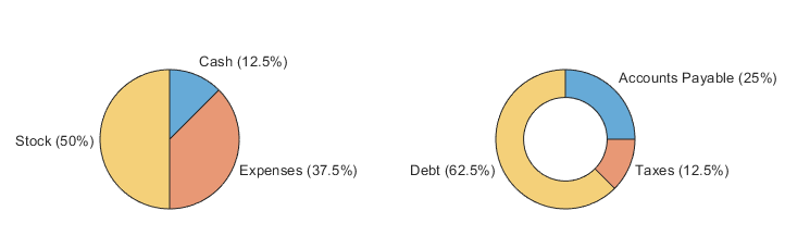
Pie chart and a donut chart

Plot Colors: Choose from nine color palettes

Plot multiple data series together using one of nine different color palettes to differentiate the individual data series. You can change the palette by passing the palette's name to the colororder function. The available names are "gem", "gem12", "glow", "glow12", "sail", "reef", "meadow", "dye", and "earth". The "gem" palette is the default for most plots.

You can also use the orderedcolors function to get the RGB triplets for any of the palettes.
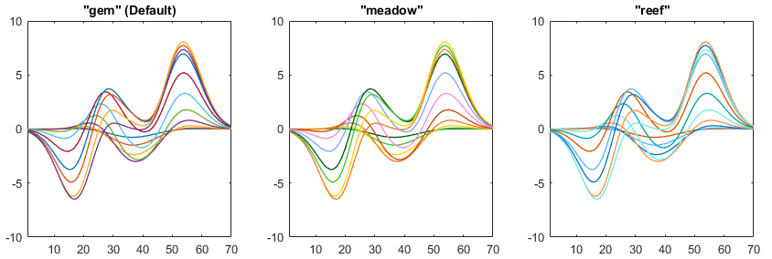
Three line plots displayed with the gem, meadow, and reef color palettes

abyss Function: Apply blue-to-black colormap to charts and images

Use the abyss function to get a blue-to-black colormap for coloring your charts. Like for all predefined colormaps, you can optionally specify the number of colors for the abyss colormap.
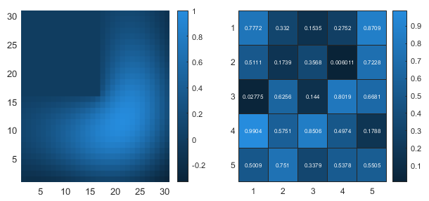
Image and a heatmap chart that use the abyss colormap

Legend: Control the order of legend entries

Control the order of legend entries by setting the Direction property of the legend to "normal" or "reverse". In most cases, the default direction is "normal".

Legends for stacked bar charts and area charts have a reverse order by default so the legend entries match the stacking order of the chart. For more information, see Legend order is reversed for stacked bar charts and area charts.
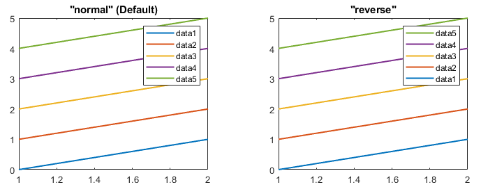
Two identical line plots that each have a legend. One legend has the default normal direction, and the other legend has the reverse direction.

xscale, yscale, and zscale Functions: Quickly change between logarithmic and linear axes scales after plotting

View any dimension of a plot on a logarithmic or linear scale by calling the xscale, yscale, or zscale function after plotting. To switch between the different scales, call any of these functions with "linear" or "log" as an input argument. For example, yscale("log") changes the scale of the y-axis to be logarithmic.
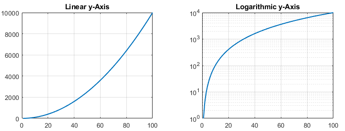
Two plots of the same data, one plot with a linear y-axis and the other plot with a logarithmic y-axis

xsecondarylabel, ysecondarylabel, and zsecondarylabel Functions: Create, delete, or modify secondary axis labels

Create, delete, or modify secondary axis labels by calling the xsecondarylabel, ysecondarylabel, and zsecondarylabel functions. Secondary labels are text labels that appear at the edge of the axes and provide additional information about the data. Often, they provide information about the units or scale of the data.

For example, create a bar chart with datetime values along the x-axis and feet along the y-axis. By default, the chart has a secondary x-axis label of "2020". Call the xsecondarylabel function with an empty string to delete the "2020" label. Then add a secondary label of "Feet" to the y-axis.

x = datetime(2020,5,1:8);
y = 100:100:800;
bar(x,y)
xsecondarylabel("");
ysecondarylabel("Feet")
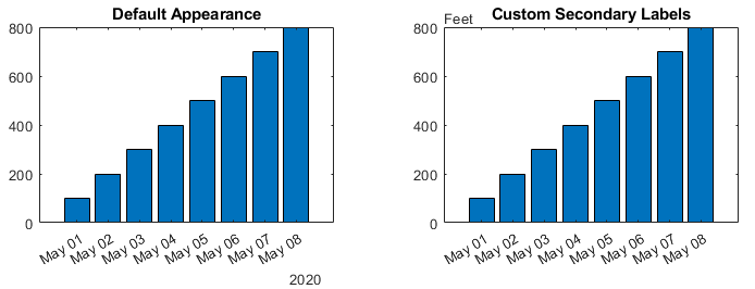
Two bar charts. One chart has the default secondary x-axis label for the datetime values and no secondary y-axis label. The other chart has no secondary x-axis label and a custom secondary y-axis label of "Feet".

Bar Charts: Specify bar labels as string vectors

When you create bar charts using the bar and barh functions, you can specify the bar labels as string vectors. The bar tick labels appear in the order you specify them.

bar(["Vanilla","Chocolate","Cherry","Almond"],[1 2 3 4])

Bar chart with the bar labels "Vanilla", "Chocolate", "Cherry", and "Almond"

xregion and yregion Functions: Create unbounded regions and specify multiple regions as matrix

Create unbounded filled regions by passing Inf or -Inf to the xregion and yregion functions. You can also create multiple regions by specifying one matrix input argument as an alternative to specifying two vectors of coordinates. For n regions, the matrix must be 2-by-n or n-by-2 and contain the lower and upper bounds for all the regions.
Line plot with three shaded regions

Text Objects: Control whether text labels are included in axes limits

Create text objects with the anchor point positions included in the axes limits calculation. To include an anchor point in the calculation, set the AffectAutoLimits property of the text object to "on".

For example, create a line plot.

x = 0:0.1:10;
y = sin(x);
plot(x,y)
Plot of a sine wave. The y-axis upper limit is 1.

Create a text object outside of the current y-axis limits. Set the AffectAutoLimits property to "on" so that the axes limits adjust to include the anchor point of the text.

text(1.1,1.1,"Peak",AffectAutoLimits="on")
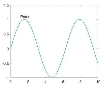
Plot of a sine wave with the text "Peak" above the first peak of the wave. The y-axis upper limit is 1.5.

Contour Plots: Customize colors of contour labels

Set the LabelColor property of a Contour object to display labels that match the colors of the contour lines, or specify one color for all the labels.
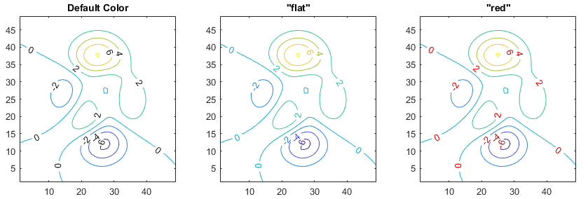
Three contour plots with different LabelColor property values. The default value displays black contour labels. A value of "flat" displays labels that match the corresponding contour lines. A value of "red" displays red labels.

Colors and Line Styles: Control automatic color and line style selection for additional chart objects

Now you can match the colors and line styles of more objects in the axes by setting the SeriesIndex property of the objects to the same value. The SeriesIndex property is available for Text, ConstantLine, ConstantRegion, Rectangle, Patch, and AnimatedLine objects, and lines created by the line, streamline, and streamslice functions.

Also, the SeriesIndex property has a new option, "none", which enables you to opt out of automatic selection for certain objects, such as reference lines.
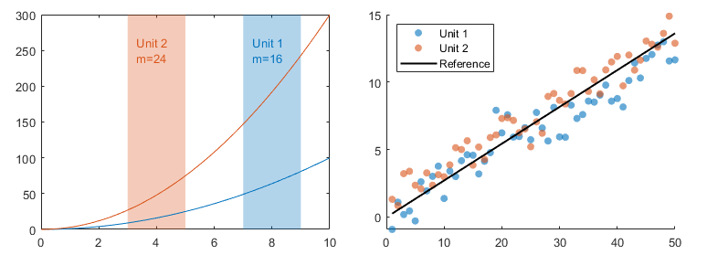
Two plots that show different ways of using the SeriesIndex property. One plot contains colored groupings of lines, filled regions, and text. The other plot contains two sets of colored scattered points with a black reference line that runs through the points.

With the new SeriesIndex property support, lines created with the line, streamline, and streamslice functions have a different default color. For more information, see Default color is different for lines created with the line function and Default color is different for plots created with the streamslice and streamline functions.

Heatmap Charts: Control text interpreter for text labels in heatmap charts

Create text, such as titles and axis labels, for heatmap charts with TeX markup, LaTeX markup, or no markup by setting the Interpreter property of the chart.
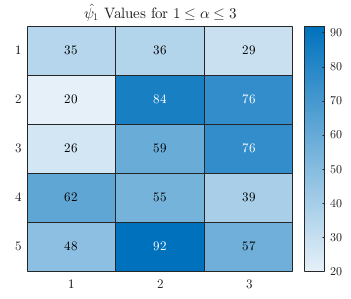
Heatmap chart with a title containing Greek letters and mathematical symbols

Images: Display images with datetime, duration, or categorical pixel coordinates

You can now display images using datetime, duration, or categorical coordinate values with the image and imagesc functions. Previously, only numeric and logical coordinate values were supported.

For example, display an image with datetime values along the x-axis and duration values along the y-axis.

x = datetime(2020,1,[1 10]);
y = minutes([1 10]);
C = peaks(10);
imagesc(x,y,C)
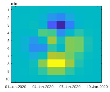
Image with x-axis tick labels that are datetime values and y-axis tick labels that are in minutes

swarmchart Function: Create horizontal swarm charts

Create a horizontal swarm chart by setting the YJitter property when you call the swarmchart function. When you specify the YJitter property without specifying the XJitter property, MATLAB sets the XJitter property to "none", and the resulting distributions in the chart are horizontal.
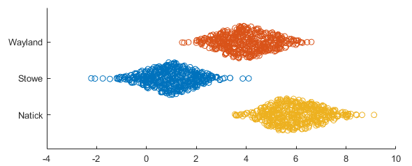
Horizontal swarm chart of three distributions of points

Geographic Plots: Some basemaps have improved appearance at high zoom levels

The "streets-light", "streets-dark", "streets", and "topographic" basemaps hosted by Esri, which are used by geographic axes objects and other objects with a Basemap property, have an improved visual appearance at high zoom levels. For example, this image compares a basemap at zoom level 21 in R2023a with the same basemap and zoom level in R2023b.
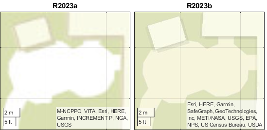
Comparison of basemaps in R2023a and R2023b. The basemap in R2023b shows crisper lines than the basemap in R2023a.

The basemaps can also have different appearances at other zoom levels. For example, this image compares a basemap at zoom level 15 in R2023a with the same basemap and zoom level in R2023b.
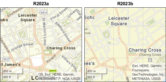
Comparison of basemaps in R2023a and R2023b. The basemap in R2023b shows fewer street names than the basemap in R2023a.

For more information about changing the basemap of geographic axes, see geobasemap.

The basemaps hosted by Esri update periodically. As a result, you might see differences in your visualizations over time.

Figure Code in MATLAB Online: Generate code from Camera tab

For a 3-D figure in MATLAB Online, when you change the camera view using the Camera tab, MATLAB generates code for the camera motion. On the Tools tab of the figure window, click Camera Tools to open the Camera tab. Use the controls in the Camera tab to interactively change the camera view. Then, to view or copy the generated code, select Show Code in the File section of the Figure tab.

Previously, MATLAB did not generate code when changing the camera view using the Camera tab.

Figure Code in MATLAB Online: Generate code from Property Inspector

For a figure in MATLAB Online, when you change the value of a graphics object property using the Property Inspector, MATLAB generates code to set the property value. On the Format tab of the figure window, click Inspect to open the Property Inspector. Use the controls in the inspector to set the value of a property. Then, to view or copy the generated code, select Show Code in the File section of the Figure tab.

MATLAB generates code only for properties that are specified as a 1-D array. Previously, MATLAB did not generate code when setting a property value using the Property Inspector.

 Functionality being removed or changed

GraphicsSmoothing and FontSmoothing properties will be removed

Still runs

The GraphicsSmoothing property of figures and the FontSmoothing property of axes, rulers, geographic scales, and text objects will be removed in a future release. All graphics will be smooth and all text will use antialiasing when these properties are removed.

spinmap function will be removed

Still runs

The spinmap function will be removed in a future release. There is no replacement for this function.

Some printing and exporting workflows will no longer support UI components

Warns

These functions and menu items will no longer support printing or exporting UI components in a future release:

  • The print function

  • The saveas function

  • The File > Save As menu item on the figure

  • The File > Export Setup menu item on the figure

  • The Edit > Copy Options menu item on the figure

To export a figure containing UI components, call the exportapp function. For example, create a simple app containing two buttons and a slider. Export the contents of the figure as a PDF file by calling the exportapp function.

% Create figure with three UI components
f = uifigure;
button1 = uibutton(f,"Position",[150 300 100 50]);
button2 = uibutton(f,"Position",[300 300 100 50]);
slider1 = uislider(f,"Position",[150 250 250 3]);

% Export the contents of the figure
exportapp(f,"myapp.pdf")

Alternatively, call the getframe function to capture the contents of the figure. Then call the imwrite function to save the content. This time, save the content as a JPEG file.

F = getframe(f);
imwrite(F.cdata,"myapp.jpg");

Exporting workflows will no longer support BMP, HDF, PBM, PCX, PGM, and PPM files

Warns

These functions and menu items will no longer support BMP, HDF, PBM, PCX, PGM, and PPM files in a future release:

  • The print function

  • The saveas function

  • The File > Save As menu item on the figure

  • The File > Export Setup menu item on the figure

To export graphics using one of these formats, use the imwrite function instead. For example, create a line plot, and capture the contents of the current figure using the getframe function. Then save the content as a BMP file.

plot([0 3 2 4 1]);
F = getframe(gcf);
imwrite(F.cdata,"myplot.bmp");

Some exporting workflows will no longer support PostScript (.ps) files

Warns

These functions and menu items will no longer support creating full-page PostScript (.ps) files in a future release:

  • The print function

  • The saveas function

  • The File > Save As menu item on the figure

  • The File > Export Setup menu item on the figure

To export graphics files, call the exportgraphics function. Specify an .eps, .pdf, or .emf file extension, and set the ContentType name-value argument to "vector". This function captures content that is tightly cropped around plots, and it does not create full-page output. For example, create a plot and save the contents of the current figure as a PDF file containing vector graphics.

plot([0 3 2 4 1]);
exportgraphics(gcf,"myplot.pdf",ContentType="vector")

Alternatively, call the print function and specify an .eps, .emf, or .svg file extension. For example, create a plot and save the contents of the current figure as an EPS file.

plot([0 3 2 4 1]);
print("myplot.eps","-depsc")

The getframe function will no longer capture the figure toolbar, menu bar, or borders

Warns

In a future release, the getframe function will no longer support capturing the figure toolbar, menu bar, or the border around the figure using the rect argument. You will still be able to define a subsection of the figure to capture, but the toolbar, menu bar, and borders will not be included.

As an alternative, you can use the exportapp function to capture the toolbar and menu bar, but not the borders.

printopt will be removed

Warns

The printopt function will be removed in a future release. To configure printer defaults, use the options provided by your operating system.

Legend order is reversed for stacked bar charts and area charts

Behavior change

The default order of legend entries for stacked (vertical) bar charts and area charts is now reversed to match the stacking order of the chart. Previously, the legend entries were listed in the opposite order of stacked bars and area charts.

To preserve the order of previous releases, set the Direction property of the legend to "normal".

lgd = legend;
lgd.Direction = "normal";
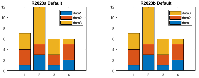
Comparison of default legends for stacked bar charts in R2023a and R2023b. The legend in R2023b has a reverse direction, which matches the stacking order of the bars.

Default color is different for lines created with the line function

Behavior change

Now that the SeriesIndex property is available for lines created with the line function, the lines cycle through the same colors (and optional line styles) that most other plots do.

The default color change applies only to the lines you create when you specify the x, y, and optional z arguments. If you create lines with a syntax that uses name-value arguments only, the plots look the same as in previous releases.

For example, create two lines with x and y input arguments. In R2023b, the first line is blue and the second line is red-orange. Before R2023b, both lines were blue.

line1 = line([0 1],[0 1]);
line2 = line([0 1],[1 2]);
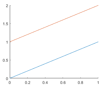
A blue line and a red-orange line plotted together

To preserve the behavior of previous releases, set the SeriesIndex property of the lines to 1. You can set the property using a name-value argument when you call the line function, or you can set the property of the Line object using dot notation later.

% Use a name-value argument
line1 = line([0 1],[0 1],SeriesIndex=1);
 
% Use dot notation
line2 = line([0 1],[1 2]);
line2.SeriesIndex = 1;
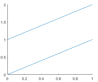
Two blue lines plotted together

Default color is different for plots created with the streamslice and streamline functions

Behavior change

When you create a streamslice or streamline plot, MATLAB automatically assigns colors and line styles the same way as for most other plots. For example, the first set of lines created with streamslice are now a soft blue color.

[x,y] = meshgrid(-10:10);
u = 2.*x.*y;
v = y.^2 - x.^2;
slicelines = streamslice(x,y,u,v);
axis tight
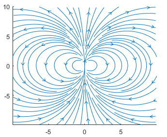
streamslice plot that has soft blue streamlines

If you call either of the functions repeatedly, subsequent plots cycle through the same set of colors as other plots do. In previous releases, the lines were bright blue.

To preserve the appearance from previous releases, use the set function to set the Color property to [0 0 1].

set(slicelines,Color=[0 0 1])
streamslice plot that has bright blue stream lines

RotateStyle property of a rotate3d object will have no effect

Behavior change in future release

The RotateStyle property of a rotate3d object will have no effect in a future release. Plot-box outline rotation will no longer be supported, and rotation will be about the entire axes regardless of the value of the property.

App Building

uislider Function: Create slider to specify range of values in apps and on App Designer canvas

You can create a range slider using the uislider function by specifying the style as "range". Alternatively, in App Designer, you can drag a Slider (Range) component from the Component Library onto the canvas. The range slider has two thumbs that app users can use to adjust the range of values. For example, this code creates a range slider that specifies values from 10 to 60.

fig = uifigure;
sld = uislider(fig,"range",Value=[10 60]);
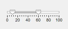
Range slider with one thumb at 10 and one thumb at 60

uicontextmenu and uimenu Functions: Access information about action used to open context menu

You can now more easily customize and share context menus in an app by using callback event data. The ContextMenuOpeningFcn and MenuSelectedFcn callbacks have additional event data when the callback is associated with a context menu on a UI component.

Event Data PropertyDescription
ContextObjectObject that the app user right-clicked to open the context menu
InteractionInformationInformation about where in the component the app user right-clicked to open the context menu, such as the cell of a table

For more information, see ContextMenu Properties and Menu Properties.

uispinner and uieditfield Functions: Create spinners and numeric edit fields with placeholder text

Create a spinner or numeric edit field that has an empty value by setting the AllowEmpty property to "on" and the Value property to []. The component appears with no default value. You can specify placeholder text to give app users a hint about the type of content the field accepts by using the Placeholder property.

For more information, see Spinner Properties and NumericEditField Properties.

uilistbox and uidropdown Functions: Access index of component value in list of items

Access the index of the value in a list box or drop-down component by using the ValueIndex property. This property is useful when the component has information stored in both the Items and ItemsData properties and you need to:

  • Query both the current item and its associated data.

  • Specify a new value using the index of the value in the list of items.

For example, use the ValueIndex property to display both the current item and its associated data.

fig = uifigure;
dd = uidropdown(fig, ...
    Items=["Apple","Banana","Cherry"], ...
    ItemsData=[0.5 0.2 1.3]);
idx = dd.ValueIndex;
 
disp(dd.Items(idx) + ": " + dd.Value)
Apple: 0.5

For more information, see ListBox Properties and DropDown Properties.

uitable Function: Query selected table data in current table display

When you create a table, use the DisplaySelection property of the table to query the cells that are selected in the current table display. This property is useful when an app user has sorted or rearranged columns in the table and you want to know which cells are selected based on the app user's view of the data.

For more information, see Table Properties.

 uicontextmenu Function: Context menus on trees appear when you right-click anywhere in the tree

When you create a context menu and assign it to a Tree object, the context menu appears when you right-click anywhere in the tree, including the area with tree nodes. You can share a single context menu across all nodes in a tree by setting the context menu on the tree instead of each individual tree node.

If you set a context menu on an individual TreeNode object, the tree node context menu still appears when you right-click the node, even if the Tree object has an assigned context menu.

 Compatibility Considerations

Previously, context menus on trees appeared only when you right-clicked on the portion of the tree below the tree nodes. To retain this behavior, create a ContextMenuOpeningFcn callback that shows the context menu only when the right-click occurs on a region without a tree node.

fig = uifigure;
cm = uicontextmenu(fig,ContextMenuOpeningFcn=@hideMenu);
m1 = uimenu(cm,Text="Menu Item");
t = uitree(fig,ContextMenu=cm);
n1 = uitreenode(t);
 
function hideMenu(src,event)
if isprop(event.InteractionInformation,"Node")
    src.Visible = "off";
end
end

appmigration.migrateGUIDEApp Function: Migrating multiple apps from GUIDE to App Designer updates app references

When you use the appmigration.migrateGUIDEApp function to migrate multiple apps at once from GUIDE to App Designer, the function updates app references. For example, to migrate a main app that opens a secondary app from GUIDE to App Designer, first download the GUIDE to App Designer Migration Tool for MATLAB. Then, use the appmigration.migrateGUIDEApp function to migrate the main and secondary apps using a single command. The function replaces all references to the apps that you migrate together. Therefore, your migrated main app opens the migrated secondary app without any manual changes to your app code.

App Designer: Interactively rearrange tabs, menus, tree nodes, and toolbar tools

Interactively rearrange tabs, menus, tree nodes, and toolbar tools between parents by dragging the component in the Component Browser. For example, interactively move and change the parents of menus and menu items.
Animation of rearranging menu items in App Designer by dragging the menu components in the Component Browser

App Designer: Write unit tests for custom UI components

You can write unit tests for custom UI components created in App Designer by using the app testing framework. To enable the unit tests to access the underlying UI components in your custom component, with the custom component open in App Designer, select the component node in the Component Browser and select Give Test Cases Access in the Testing section. Then, reference the underlying UI components in your unit tests to test the component behavior.

Running tests for custom UI components interactively using matlab.unittest.TestCase.forInteractiveUse is not supported.

For more information, see Write Tests for Custom UI Component.

App Designer: View changes to HTML UI component source while working in Design View

While designing an app that contains an HTML UI component, you can now more easily see updates made to the HTML source. To show the most up-to-date content in Design View when the HTMLSource property of the component is a path to an HTML source file, click Refresh Source while pointing to the HTML UI component in the canvas.

For more information about using HTML UI components, see Create HTML Content in Apps.

Comparison Tool: Save app comparison results as PDF or DOCX reports programmatically and interactively

You can now use the Comparison Tool to programmatically and interactively publish App Designer app comparison results as PDF or DOCX reports. For more information, see visdiff.

Axes Interactions: Interpolate data tip location

For axes in apps created in App Designer or using the uifigure function, control the method for placing data tips by using the InteractionOptions property of the axes. Create data tips at the closest interpolated location on the plot to the cursor location by setting the DatatipsPlacementMethod property of the InteractionOptions object to "interpolate". By default, data tips are created at the closest data point to the cursor location.

Axes Interactions: Indicate azimuth and elevation angles

For axes in apps created in App Designer or using the uifigure function, indicate the azimuth and elevation angles during interactive rotation by using the InteractionOptions property of the axes. The azimuth and elevation angles define the camera line of sight and are displayed when the RotateIndicator property of the InteractionOptions object is set to "azimuthelevation". By default, the axes do not display the azimuth and elevation angles.

Axes Interactions: Zoom into rectangular region of 2-D view of 3-D chart

For a 2-D view of a 3-D chart in apps created in App Designer or using the uifigure function, you can zoom into a rectangular region. To enable region-zooming, click the Zoom In or Zoom Out button in the axes toolbar, or set the Interactions property of the axes to the regionZoomInteraction object.

For example, create a 3-D surface plot and set the view to the x- and z-axes. Click the Zoom In button and then drag to select the region of interest.

f = uifigure;
a = axes(f);
surf(a,peaks);
view(a,[0 0]);
xz view of a 3-D surface plot with zoom mode enabled. A mouse cursor drags to select a rectangular region of interest.

Previously, for 3-D charts, the region-zoom interaction was supported only for the xy view.

App Testing Framework: Automatically scroll to components outside viewable area

If you programmatically perform a gesture on a UI component that is not in the viewable area of an app, the app testing framework automatically scrolls to the specified component before performing the gesture. For the framework to bring the component into view, the component must be supported by the scroll function and all its ancestors must have their Scrollable property set to "on" or true. For example, create a scrollable figure with a state button that is outside the viewable area of the figure, and then press the button.

fig = uifigure(Scrollable="on");
b = uibutton(fig,"state",Position=[fig.Position(3)+100 100 100 22]);

testCase = matlab.uitest.TestCase.forInteractiveUse;
testCase.press(b)

Web Apps and Standalone Applications: Data brushing supported in graphics

Graphics created in web apps and standalone applications support data brushing. Use data brushing in these applications just as you would in MATLAB figures.

Performance

Language and Programming: Improved performance for reading and writing class property values

Reading and writing class property values shows improved performance. The largest gains in performance are for accessing properties that do not use validation or get and set methods.

For example, the movingAverage method of StorageClass reads several elements from the data property and writes to the average property.

classdef StorageClass
    properties
        data
        average
        N
    end
    methods
        function obj = StorageClass(dataIn)
            obj.data = dataIn;
            obj.N = numel(dataIn);
            obj.average = zeros(1, obj.N-2);
        end
        function obj = movingAverage(obj)
            for ix = 1:(obj.N-2)
                obj.average(ix) = (obj.data(ix) +...
                    obj.data(ix+1) + obj.data(ix+2))/3;
            end
        end
    end
end

This code is about 17.5x faster than in the previous release.

s = StorageClass(1:1e6);
timeit(@()s.movingAverage)

The approximate execution times are:

R2023a: 0.497 s

R2023b: 0.0284 s

The code was timed on a Windows 10, Intel Xeon CPU E5-1650 v3 @ 3.50 GHz test system.

dde23 Function: Improved performance integrating high-dimensional systems

The dde23 function shows improved performance solving high-dimensional systems of DDEs over long integration intervals. The improvement gets better as the number of coupled DDEs in the system increases.

For example, this code solves a system of 500 coupled DDEs over the time interval [0 100]. The code is about 24x faster than in the previous release.

function timingdde23
rng default
N = 500; 
C = rand(N); 
lag = 1; 
dderhs = @(t,y,ylag) -y-C*ylag; 
sol = dde23(dderhs,lag,10+rand(1,N),[0 100]); 
end

The approximate execution times are:

R2023a: 5.6 s

R2023b: 0.23 s

The code was timed on a Windows 10, Intel Xeon CPU W-2133 @ 3.60 GHz test system using the timeit function.

timeit(@timingdde23)

nufftn Function: Improved performance with nonuniform sample points or query points

The nufftn function shows improved performance when operating on either nonuniformly spaced sample points or nonuniformly spaced query points.

For example, this code constructs a 262,144-by-3 matrix of nonuniform sample points t and calculates the nonuniform discrete Fourier transform along each dimension of a 64-by-64-by-64 array. The code is about 3.3x faster than in the previous release.

function timingSamplePoints
rng default
t = rand(64^3,3);
X = rand(64,64,64);
tic
  Y = nufftn(X,t);
toc
end

The approximate execution times are:

R2023a: 0.40 s

R2023b: 0.12 s

The code was timed on a Windows 10, Intel Xeon CPU E5-1650 v4 @ 3.60 GHz test system by calling the timingSamplePoints function.

As another example, this code constructs a 262,144-by-3 matrix of nonuniform query points f and calculates the nonuniform discrete Fourier transform along each dimension of a 64-by-64-by-64 array. The code is about 1.6x faster than in the previous release.

function timingQueryPoints
rng default
f = rand(64^3,3);
X = rand(64,64,64);
tic
  Y = nufftn(X,[],f);
toc
end

The approximate execution times are:

R2023a: 0.40 s

R2023b: 0.25 s

The code was timed on a Windows 10, Intel Xeon CPU E5-1650 v4 @ 3.60 GHz test system by calling the timingQueryPoints function.

fillmissing Function: Improved performance when filling entries with previous or next numeric value

The fillmissing function shows improved performance when you specify the fill method as "previous" or "next" for numeric data.

For example, this code fills the NaN values in a 1000-element numeric vector with the previous nonmissing value. The code is about 6.9x faster than in the previous release.

function timingFillmissing
A = rand(1000,1);
idx = randperm(1000,50);
A(idx) = NaN;
for i = 1:2e4
    F = fillmissing(A,"previous");
end
end

The approximate execution times are:

R2023a: 1.59 s

R2023b: 0.23 s

The code was timed on a Windows 10, Intel Xeon CPU E5-1650 v4 @ 3.60 GHz test system using the timeit function.

timeit(@timingFillmissing)

ismember Function: Improved performance with small unsorted set array

The ismember function and other set operations that call ismember show improved performance when the set array is unsorted and the product of the numbers of elements in the query array and the set array is less than 256.

For example, this code returns an array containing logical 1 (true) where the data in a 6-element query array is found in a 25-element set array. The code is about 2.9x faster than in the previous release.

function timingIsmember
a = [1 2 3 4 5 6];
b = magic(5);
for i = 1:1e5
    Lia = ismember(a,b);
end
end

The approximate execution times are:

R2023a: 0.70 s

R2023b: 0.24 s

The code was timed on a Windows 10, Intel Xeon CPU E5-1650 v4 @ 3.60 GHz test system using the timeit function.

timeit(@timingIsmember)

islocalmax and islocalmin Functions: Improved performance when finding local minima and maxima

The islocalmax and islocalmin functions show improved performance. The improvement is most significant for data with large flat regions at the local maxima or minima, respectively.

For example, this code finds the local maxima of data that contains consecutive maxima values. The code is about 2.8x faster than in the previous release.

function timingIslocalmax
x = repelem([0.5 0 1 0 1 0 1 0 0.5],10000);
for i = 1:3e2
    TF = islocalmax(x);
end
end

The approximate execution times are:

R2023a: 0.91 s

R2023b: 0.32 s

The code was timed on a Windows 10, Intel Xeon CPU E5-1650 v4 @ 3.60 GHz test system using the timeit function.

timeit(@timingIslocalmax)

Data Cleaner App: Improved rendering performance of Cleaning Parameters panel

In the Data Cleaner app, the Cleaning Parameters panel renders more quickly after selecting a cleaning method in R2023b than in R2023a. The delay before you can interact with the panel is reduced.

For example, if one table variable is selected in the Data Cleaner app and you select the Clean Outlier Data cleaning method, the Cleaning Parameters panel is ready about 1.14x faster in R2023b than in the previous release.

The approximate panel rendering times are:

R2023a: 2.4 s

R2023b: 2.1 s

The panel rendering was timed on a Windows 10, Intel Xeon CPU E5-1650 v4 @ 3.60 GHz test system by selecting the cleaning method in the Data Cleaner toolstrip and measuring the time it takes for the Cleaning Parameters panel to be ready.

Tiled Chart Layouts: Improved performance for flow layouts with spanned axes

Tiled chart layouts that have the "flow" tile arrangement and axes that span many tiles are more responsive when the tile arrangement changes. The tile arrangements change under these conditions:

  • Adding new axes

  • Resizing the figure

  • Customizing the appearance of the axes by setting axes properties

For example, this code is about 1.4x faster than in the previous release.

function mylayout
tiledlayout("flow")
for i = 1:6
    nexttile([1000,1000]);
end
end
3-by-2 grid of axes in a tiled chart layout

The approximate execution times are:

R2023a: 0.0380 s

R2023b: 0.0276 s

The code was timed on a Windows 10, Intel Xeon CPU W-2133 @ 3.60 GHz test system using the timeit function.

timeit(@mylayout)

Plots in Apps: Improved performance when scrolling to zoom

Zooming using a multi-touch trackpad or mouse shows improved performance in plots within apps and within figures created using the uifigure function. The two-finger scroll gesture and the zooming action are more synchronized in R2023b than in R2023a. The improvement results in a smoother experience when zooming.

For example, this code creates a figure with a plot of random data. On a Windows 10, Intel Xeon CPU E5-1650 v4 @ 3.60 GHz test system, when you zoom into the plot using the two-finger scroll gesture on a trackpad, the plot rendering is smoother and the zooming speed is more precise, especially at slower speeds, in R2023b than in the previous release.

f = uifigure;
ax = uiaxes(f);
plot(ax,magic(10))

Plots in Apps: Improved responsiveness for scatter plot interactions in apps

Interactions with scatter plots show improved responsiveness. To observe the improvement, the plot must be created in an app or in a figure created with the uifigure function, and the markers must either be points (".") or have a size less than 35. The improvement is most noticeable for plots with 1 million or more points.

For example, on a Windows 10, Intel Xeon CPU W-2133 @ 3.60 GHz test system, create a 3-D scatter plot with 7 million points in an app window, and then drag to rotate the axes. The rotation is smoother and responds more quickly to the drag gesture in R2023b than in the previous release.

function myscatter
f = uifigure;
ax = axes(f);
z = linspace(0,4*pi,7e6);
x = 2*cos(z) + rand(1,7e6);
y = 2*sin(z) + rand(1,7e6);
scatter3(ax,x,y,z,[],1:7e6,".")
end

These animations start with the corner of the xy-plane at (–2, –2) in the center of the frame.

R2023a

R2023b

The rotation of the axes lags behind the movement of the cursor.

Animation of a rotating 3-D scatter plot in R2023a

The rotation of the axes is smoother and follows the movement of the cursor more closely.

Animation of a rotating 3-D scatter plot in R2023b

Plots in Apps: Constant lines and constant regions update continuously as you pan

In apps, panning a plot containing ConstantLine or ConstantRegion objects is smoother and the contents of the axes update immediately as you pan. Previously, panning showed blank areas when you panned outside of the original axes limits.

For example, on a Windows 10, Intel Xeon CPU W-2133 @ 3.60 GHz test system, if you run this code and then pan within the axes, the horizontal line and the gray vertical region update immediately as you pan.

function myapp
fig = uifigure;
ax = axes(fig);
x = -10:0.1:10;
y = sin(x);
plot(ax,x,y);
xlim(ax,[-6 6])
yline(ax,0)
xregion(ax,-3,3)
end

R2023a

R2023b

The plot shows blank areas during the panning interaction.

Animation of panning within a plot containing a constant line and a constant region in R2023a

The plot updates immediately during the panning interaction.

Animation of panning within a plot containing a constant line and a constant region in R2023b

App Building: Improved performance when resizing apps with nested containers

When a user resizes an app figure window for the first time, many apps reposition their content significantly faster in R2023b than in R2023a. The improvement occurs when resizing an app with one or more containers that have the AutoResizeChildren property set to "on", which is the default value. The improvement is more noticeable for apps with nested containers, such as apps with many tabs or tab groups.

For example, this code creates an app that contains five top-level tabs, each of which contains five nested tabs. Each of the nested tabs contains 100 edit fields. When you run this app and resize it, the resize operation is about 30x faster in R2023b than in the previous release.

function myApp
f = uifigure;
f.Position = [100 100 700 500];
 
% Create five tabs in a tab group
tg = uitabgroup(f,"Position",[1 1 700 500]);
nTabs = 5;
for kTab = 1:nTabs
    tab = uitab(tg,"Title","Tab " + kTab);
    createTabContent(tab);
end
 
    function createTabContent(tab)
        % Create a nested tab group containing five tabs
        nestedTg = uitabgroup(tab,"Position",[10 10 650 450]);
        nNestedTabs = 5;
        for kNTab = 1:nNestedTabs
            nestedTab = uitab(nestedTg,"Title","Nested Tab "+ kNTab);
            % Add 100 edit fields to the tab
            createNestedTabContent(nestedTab);
        end
    end
 
    function createNestedTabContent(tab)
        % Add 100 edit fields to a tab
        hParent = 400;
        n = 10;
        w = 50;
        h = 22;
        for kRow = 1:n
            for kCol = 1:n
                uieditfield(tab,"Position",[(kCol-1)*(w+10)+10,hParent-kRow*(h+10),w,h]);
            end
        end
    end
end

R2023a

R2023b

The app takes about 60 seconds to resize.

Animation of an app resizing in R2023a. When the figure window size changes, the content in the app does not reposition within the time frame of the animation.

The app takes about two seconds to resize.

Animation of an app resizing in R2023b. When the figure window size changes, the content in the app repositions in approximately two seconds.

The resize interactions were times on a Windows 10, Intel Xeon Gold 6246R CPU @ 3.40 GHz test system by running the myApp function and measuring the time it takes for the figure window to resize.

App Building: Improved startup performance for apps with panels in multiple tabs

In addition to the overall app startup performance improvement in R2023b, some apps that contain panels in multiple tabs show an even greater startup performance improvement. The reason is that MATLAB prioritizes creating the panel content in the visible tab over non-visible content when the app first runs.

For example, this code creates a tab group with five tabs, each containing a panel with 200 label components. The code is about 1.2x faster than in the previous release.

function timingTabApp
fig = uifigure;
tg = uitabgroup(fig); 
for k1 = 1:5
    t = uitab(tg);
    p = uipanel(t,Position=[1 1 t.Position(3) t.Position(4)], ...
        Scrollable="on");
    for k2 = 1:200
        y = k2*20;
        uilabel(p,Position=[20 y 60 20]);
    end
end
end

The approximate execution times are:

R2023a: 7.2 s

R2023b: 6.1 s

The code was timed on a Windows 10, Intel Xeon CPU E5-1650 v4 @ 3.60 GHz test system by running the timingTabApp function and measuring the time it takes for the components to appear in the UI figure window.

If you have an app with many UI components, consider updating your app layout to take advantage of this improvement. For more information, see Improve App Startup Time.

App Designer: Improved app loading and running performance

Loading existing apps in App Designer is faster in R2023b than in R2023a. When you load an App Designer app, it takes less time for the app to appear in Design View.

For example, loading an app with about 400 UI components by selecting the app file on the App Designer Start Page is about 1.3x faster than in the previous release.

The approximate load times are:

R2023a: 17.1 s

R2023b: 13.6 s

In addition, running an app from App Designer is also faster in R2023b.

For example, for an app with about 400 UI components, running the app by clicking the Run button in App Designer results in the app appearing about 1.3x faster than in the previous release.

The approximate execution times are:

R2023a: 25.5 s

R2023b: 19.3 s

The actions were timed on a Windows 10, Intel Xeon CPU E5-1650 v4 @ 3.60 GHz test system by loading and running a saved app.

App Designer: Improved performance when adding custom UI components to an app

When you drag a custom UI component from the Component Library onto the App Designer canvas, the UI component appears sooner in R2023b than in R2023a. This improvement is more noticeable the first time you add a custom UI component to an app.

For example, on a Windows 10, Intel Xeon CPU E5-1650 v4 @ 3.60 GHz test system, the first time you add a custom UI component to an app in Design View, the component appears on the canvas within one second. In R2023a, the component takes several seconds to appear.

Property Inspector in MATLAB Online: Improved performance when opening for the first time

The Property Inspector shows improved performance when opening for the first time in MATLAB Online. The delay between clicking the Property Inspector icon or calling inspect and the inspector being ready is reduced.

For example, open the Property Inspector for the first time in MATLAB Online. You can use the Property Inspector 1.8x sooner than in the previous release.

ax = axes;
inspect(ax)

The approximate rendering times are:

R2023a: 7.5 s

R2023b: 4.1 s

The rendering of the Property Inspector was timed by running the code and measuring the time it takes for the edit fields to appear in the Property Inspector.

Graphics in MATLAB Online: Images and 3-D plots in apps have significant performance gains

Displaying images and 3-D plots in apps is significantly faster in MATLAB Online. You might also experience similar improvements outside the context of an app (by calling figure instead of uifigure).

For example, this code displays a scaled-up version of peppers.png using the image command. The code is about 22x faster than in the previous release.

function myapp
f = uifigure;
ax = axes(f);
smallimg = imread("peppers.png");
bigimg = uint8(zeros(3065,4089,3));
bigimg(:,:,1) = uint8(interp2(double(smallimg(:,:,1)),3));
bigimg(:,:,2) = uint8(interp2(double(smallimg(:,:,2)),3));
bigimg(:,:,3) = uint8(interp2(double(smallimg(:,:,3)),3));
 
tic
image(ax,bigimg)
drawnow
toc
end
peppers.png image resized to 3065-by-4089 pixels

The approximate execution times are:

R2023a: 138.5 s

R2023b: 6.4 s

The code was timed by calling the myapp function. Because MATLAB Online is hosted, performance is independent of the computer hardware used to access it.

Software Development Tools

 Source Control API: Interact with Git source control programmatically

You can now programmatically interact with source control.

  • Clone a Git repository using the gitclone function.

  • Create a Git repository object using the gitrepo function.

  • Initialize a Git repository using the gitinit function.

  • Create, delete, and switch branches using the createBranch, deleteBranch, and switchBranch functions, respectively.

  • Add files, remove files, and commit changes to a Git repository using the add, rm, and commit functions, respectively.

  • Inspect the commit history in a Git repository using the log function.

  • Display the status of files in a local Git repository using the status function.

  • Fetch or pull new data from remote Git repositories using the fetch or pull functions, respectively.

  • Merge Git branches and revisions into the current branch using the merge function.

  • Publish your local changes to a remote Git repository using the push function.

Project API: Determine whether file belongs to a project

You can now programmatically determine whether a file or a folder belongs to a project by using the matlab.project.isFileInProject function.

Source Control in MATLAB Online: Perform source control operations using unified panel

In MATLAB Online, you can use the Source Control panel to see all active source control repositories, manage modified files, and perform source control operations.
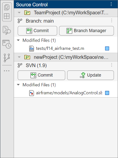
Source Control panel showing two repositories. The first repository is under Git source control and the second is under SVN source control.

To open the Source Control panel, use the Open more panels button (three-dot icon) in the sidebar.

MATLAB Online desktop with the Open more panels buttons circled in the left and bottom sidebars. The Open Panel dialog box shows the available panels.

Source Control in MATLAB Online: Expanded support for Git workflows

MATLAB Online now provides expanded support for Git workflows:

  • Adding and managing Git submodules

  • Sharing to GitHub

  • Initializing Git repositories

  • Shallow cloning Git repositories

Projects in MATLAB Online: Added support for team collaboration workflows

Projects in MATLAB Online now provide support for the following team collaboration workflows:

  • Creating referenced projects from project folders

  • Adding source control to existing projects

  • Managing project labels and custom tasks using Project Settings

  • Displaying shadowed files on project startup

  • Upgrading projects using Project Upgrade

Project Examples: Identify and run tests in projects

This example shows how to use labels to identify tests in a project and how to create test suites from project test files interactively and programmatically. For large projects under source control, the example demonstrates how to run a subset of tests to reduce qualification runtime. For more information, see Identify and Run Tests in MATLAB Projects.

 Build Automation: Use built-in tasks to define common build actions

When using the build tool, you can create common tasks more quickly and conveniently by using the classes in the matlab.buildtool.tasks package. Instead of writing code to implement tasks, instantiate the classes in this package. Each class provides the flexibility to create a task tailored to your build requirements. For an example, see Create and Run Tasks Using Build Tool.

Build Automation: Automatically open MATLAB project when running builds

If your build file is in the root folder of a MATLAB project that is not already open, the build tool automatically opens the project before running the build and then closes the project after the build runs.

Build Automation: Invoke build tool from project subfolders

You can call the buildtool command from the folder containing the build file or any of its subfolders. In previous releases, you can call buildtool only when the build file is in your current folder.

Build Automation: Operate on file collections

The matlab.buildtool.io.FileCollection class has four new methods that enable you to create file collections and operate on them:

For an example, see Replace Substring in File Collection Paths.

Build Automation: Name the inputs and outputs of tasks for incremental builds

You can use the matlab.buildtool.TaskInputs and matlab.buildtool.TaskOutputs classes to name and group the inputs and outputs of your tasks. The TaskInputs and TaskOutputs objects behave like structures, where field names are task input or output names and field values are task input or output values. Input values can be of any data type, and output values must be matlab.buildtool.io.FileCollection arrays. For an example, see Create Task with Named Inputs and Outputs.

Build Automation: Run tasks using build options

You can use build options to run tasks with the buildtool command or the run method:

  • To run the subsequent tasks upon a build environment setup or task failure, use the -continueOnFailure option of buildtool or the ContinueOnFailure name-value argument of run.

  • To specify a task to skip, use the -skip option of buildtool or the Skip name-value argument of run.

For example, run the default tasks in your build plan as well as the tasks on which they depend, and continue running the build if a failure occurs.

buildtool -continueOnFailure

Unit Testing Framework: Programmatically access code coverage results using the runtests function

You can use the runtests function to programmatically access the results of code coverage analysis for your source code. To run tests and return coverage results, specify the additional output argument of runtests as well as the ReportCoverageFor name-value argument. When you invoke runtests by specifying both these arguments, the function returns the coverage results as a matlab.coverage.Result vector. For example, run your tests and return the results of code coverage analysis for the source code in your current folder.

[testResults,coverageResults] = runtests("myTestFile.m", ...
    ReportCoverageFor=pwd)

Unit Testing Framework: Test for missing elements

The matlab.unittest.constraints.HasMissing class provides a constraint to test if an array has any missing elements. The constraint is satisfied by an array that has at least one missing element.

Unit Testing Framework: Modify test report title

You can modify the test report title when you generate a test report using a method of the matlab.unittest.plugins.TestReportPlugin or matlab.unittest.TestResult class. To modify the title, specify the Title name-value argument. For example, run your tests and generate a PDF test report with a specified title.

results = runtests("myTestFile.m");
generatePDFReport(results,Title="My Test Report")

App Testing Framework: Automatically scroll to components outside viewable area

If you programmatically perform a gesture on a UI component that is not in the viewable area of an app, the app testing framework automatically scrolls to the specified component before performing the gesture. For the framework to bring the component into view, the component must be supported by the scroll function and all its ancestors must have their Scrollable property set to "on" or true. For example, create a scrollable figure with a state button that is outside the viewable area of the figure, and then press the button.

fig = uifigure(Scrollable="on");
b = uibutton(fig,"state",Position=[fig.Position(3)+100 100 100 22]);

testCase = matlab.uitest.TestCase.forInteractiveUse;
testCase.press(b)

matlab.test.behavior.Missing Class: Test against constructor arguments that result in incompatible values

You can verify whether objects of your class created with certain constructor arguments satisfy the missing value contract in MATLAB. To test your class with a constructor argument, specify the ExtraConstructorArguments property of the matlab.test.behavior.Missing class as that argument. This property is useful when different constructor arguments result in incompatible values, such as values that cannot be concatenated or compared.

 Functionality being removed or changed

Build tool restores the current folder after running each task

Behavior change

To prevent a task from affecting subsequent tasks by changing the current folder, the build tool restores the current folder after running each task. In previous releases, the build tool does not restore the current folder after running each task.

files converts relative paths to absolute paths

Behavior change

If you create file collections with the files method, the paths of the file collections are absolute paths. Previously, the method did not convert any relative paths that you specified to absolute paths. To create file collections with relative paths, use the matlab.buildtool.io.FileCollection.fromPaths method, or use a string vector to specify an argument or property that requires file collections.

External Language Interfaces

Call MATLAB from C++: Generate output types for strongly typed methods and functions

The matlab.engine.typedinterface.generateCPP function generates output types for functions and methods in the strongly typed C++ interface. For more information, see Output Argument Validation. For an example, see Write MATLAB Code for Strongly Typed C++ Interface.

Publish C++ Interface: Support for pointer return of string and fundamental types

When publishing a MATLAB interface to a C++ library function, you can define pointer return arguments for non-const string and fundamental types. You also can specify a deleter function for both const and non-const string and fundamental pointer return types. MATLAB uses the deleter function to manage the life cycle of the memory represented by the argument.

For examples, see Define Output Pointer Argument.

Call MATLAB from .NET: Generate C# code interface for MATLAB packages, classes, and functions

The matlab.engine.typedinterface.generateCSharp function creates C# .cs files from MATLAB packages, classes, and functions. For more information, see Strongly Typed Interface for C#.

Call .NET from MATLAB: Create explicit interface view of .NET object

You can create an explicit view of a .NET object as one of its implemented interfaces using the NET.interfaceView function. Interfaces can define methods or properties that are not accessible from the .NET object directly.

Python: Support for version 3.11

MATLAB now supports CPython version 3.11, in addition to existing support for versions 3.9 and 3.10. For supported version information, see Versions of Python Compatible with MATLAB Products by Release.

Python Interface: Use of environment variable PYTHONHOME to load interpreter

MATLAB accesses these settings when loading the Python interpreter:

  • User settings for the Python environment, configured using the pyenv function. If the version you specify conflicts with the version specified by PYTHONHOME, then delete the environment variable before calling pyenv. The value set by pyenv is persistent across MATLAB sessions. For more information, see Set Python Version on Windows Platform or Set Python Version on Mac and Linux Platforms.

  • PYTHONHOME environment variable, specifies where to find the standard Python libraries. To view the value of the variable in MATLAB, type getenv("PYTHONHOME"). For more information, see Use PYTHONHOME Environment Variable.

  • System PATH environment variable. To view the system path in MATLAB, type getenv("PATH").

  • Windows registry.

Python Interface: Convert list and tuple of Python datetime or timedelta objects to MATLAB arrays

If a Python function returns multiple datetime objects as a list or a tuple of Python datetime objects, use the MATLAB datetime function to convert the list or tuple to a MATLAB datetime array. For more information, see Handle Multiple Python datetime Objects Returned from Python Function.

If a Python function returns multiple timedelta objects as a list or a tuple of Python timedelta objects, use the MATLAB duration function to convert the list or tuple to a MATLAB duration array. For more information, see Handle Multiple Python timedelta Objects Returned from Python Function.

Python Interface: Resolve Python configuration issues

Error messages provide additional help for you to resolve these Python configuration issues:

 Compilers: Download MinGW-w64 8.1 from Add-On Explorer

As of R2023b, you can download MinGW-w64 8.1 from the Add-On Explorer.

To download or configure other supported versions of MinGW, see MATLAB Support for MinGW-w64 C/C++ Compiler. For an up-to-date list of supported compilers, see Supported and Compatible Compilers.

Compilers: Support for NAG Fortran on Apple silicon

MATLAB supports the NAG® Fortran compiler on Apple silicon platforms. For an up-to-date list of supported compilers, see Supported and Compatible Compilers.

Compilers: Support for Microsoft Visual Studio Build Tools

MATLAB supports Build Tools for Visual Studio 2022 and 2019 for building C and C++ interfaces, MEX files, and standalone MATLAB engine and MAT-file applications on Windows platforms. For an up-to-date list of supported compilers, see Supported and Compatible Compilers.

 Functionality being removed or changed

Python: Version 3.8 is no longer supported

Errors

Support for Python version 3.8 is discontinued. For continued support for your applications, upgrade to a supported version of Python. For supported version information, see Versions of Python Compatible with MATLAB Products by Release.

Perl: MATLAB support for version 5.38.0 on Windows

Behavior change

As of R2023b, MATLAB on Windows ships with an updated version of Perl, version 5.38.0, and supports an updated version of HTML::Parser, version 3.81.

If you use the perl command on Windows platforms, see https://www.perl.org/ for information about using this version of the Perl programming language. For a standard distribution of HTML::Parser, source code, and information about using HTML::Parser, see https://metacpan.org/pod/HTML::Parser.

Hardware Support

Support for ArduCam Multi Camera Adapter Module on Raspberry Pi Hardware

Starting in R2023b, you can use the new arducam object to set up a connection between MATLAB and ArduCam Multi Camera Adapter Module V2.2. You can sequentially acquire images from up to four cameras attached to the ArduCam Multi Camera Adapter Module V2.2. Raspberry Pi Blockset supports 5MP OV5647 cameras, which are compatible with ArduCam Multi Camera Adapter Module V2.2.

R2023a

New Features, Bug Fixes, Compatibility Considerations

Environment

 MATLAB Install: Reduce footprint using default installation without local documentation

Starting in R2023a, the documentation is not installed as part of a MATLAB or other product installation. This change significantly reduces the installation footprint of products. In most cases, not installing the documentation has no effect on the availability of documentation, as the Help Center displays the web documentation by default.

 Compatibility Considerations

The documentation is not installed as part of a product installation. If you run MATLAB on a system with no internet connection (permanently offline), or if you plan to work offline occasionally on an otherwise internet-connected machine, you can install the documentation on your computer after installing products. For more information, see Install Documentation.

Editor: Interactively increment numeric values within section and run section after every change

You can increment, decrement, multiply, or divide numeric values in the Editor and then run the current section after every change. This workflow can help you fine-tune and experiment with your code.

To adjust a numeric value, select the value or place your cursor next to the value. Next, right-click and select Increment Value and Run Section. In the dialog box that appears, specify a step value for addition and subtraction or a scale value for multiplication and division. Then, click one of the operator buttons to add to, subtract from, multiply, or divide the selected value in your section. MATLAB runs the section after every click.
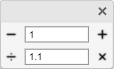
Increment Value and Run Section dialog box with the step value for addition and subtraction set to 1 and the scale value for multiplication and division set to 1.1

Live Editor Controls: Add file browser to select file interactively in live script

You can add a file browser to your live script to interactively select a file by opening a file selection dialog box. To add a file browser, go to the Live Editor tab, and in the Code section, click Control. Then, select File Browser.

File browser with the file C:\Work\data1.mat selected, assigned to the variable filename

For more information, see Add Interactive Controls to a Live Script.

Live Editor Controls: Align controls within a section when code is hidden

The Live Editor automatically left-aligns drop-down lists, edit fields, numeric sliders, and numeric spinners within a block of code when the code is hidden.

For example, this live script contains three controls in two different blocks of code. When the code is visible, the controls appear inline with the code.
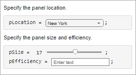
Live script with a drop-down list, slider, and edit field all in different positions within their respective code lines

When the code is hidden, the Live Editor automatically aligns the second and third controls, as they are in the same block of code. The first control is not in the same block of code and is therefore not aligned to the other two controls.
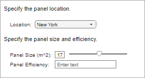
Live script with the code hidden and a drop-down list, slider, and edit field aligned to each other

The Live Editor does not align check boxes, buttons, and file browsers.

Desktop Layout in MATLAB Online: Access desktop tools and change the desktop layout using sidebars

The MATLAB Online desktop includes sidebars on either side of the desktop to access desktop tools and change the desktop layout. The sidebars show the tools, such as the Workspace panel and the Files panel, that are docked on either side of the desktop. If there are no tools docked on one side, the sidebar for that side is hidden. You can use the sidebars to show and hide tools, group them together, and move them from one location to another.

When a tool is docked on the left or right side of the desktop, the sidebar on that side displays an icon for the tool. To show or hide the tool, click its icon in the sidebar. To show and hide multiple tools together, group them by dragging one of the tool icons next to another tool icon. To move a tool to a different location on the desktop, drag the tool or the icon for the tool to the new location. If there are no tools docked on one side, then the sidebar on that side is hidden.
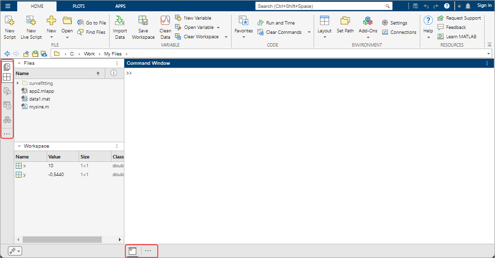
MATLAB Online desktop with two tool icons grouped together in the left sidebar. The Files panel and the Workspace panel are open on the left side of the desktop.

Code Issues Tool in MATLAB Online: Check code for errors and warnings using Code Issues tool

You can use the Code Issues tool to view error and warning messages about your code. The Code Issues tool displays the coding problems found by the MATLAB Code Analyzer as it automatically checks your code. Using the Code Issues tool, you can choose to view the errors and warnings for the current file or for all open files. You also can filter the list of messages by type (error or warning) as well as by message text.

To open the Code Issues tool, go to the Editor or Live Editor tab, and in the Analyze section, click Code Issues. By default, the Code Issues tool opens on the right side of the desktop. To hide the Code Issues tool, click the Code Issues icon in the sidebar.

Code Issues tool showing 0 errors and 13 warnings found in the lengthofline.m file. The MATLAB Online desktop right sidebar shows the Code Issues icon.

Find Files Tool in MATLAB Online: Search for files with improved Find Files tool

You can use the improved Find Files tool to search for files based on name or content. When searching, you can choose whether to match the case of your search text as well as whether to match the whole word. You also can select what folder to search in and filter results by file extension. To search for files, click the Find Files icon in the sidebar on the left side of the MATLAB Online desktop.
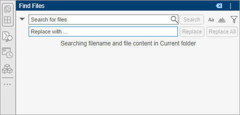
Find Files tool with a Search box and options to match the case of the search text, match the whole word, and filter results. The MATLAB Online desktop left sidebar shows the Find Files icon.

Editor in MATLAB Online: Edit read-only files

You can now edit read-only files in MATLAB Online. When you save the file, MATLAB prompts you to overwrite the file or save the file using a different name.

Search in MATLAB Online: Access videos using Search box

In MATLAB Online, you can now use the Search box in the upper-right corner of the desktop to easily access videos that show you how to use MathWorks products. In addition to videos, the Search box results include toolstrip actions, preferences, and Help Center resources such as functions, blocks, examples, and answers. To navigate to the Search box using a keyboard, press Ctrl+Shift+Space (or Command+Shift+Space on macOS systems).

System Command Functions: Set and get multiple variables using operating system commands

Set and get multiple environment variables using the setenv, unsetenv, getenv, and isenv functions with string arrays and cell arrays of character vectors as input.

loadenv Function: Load environment variables from .env and plain text files

You can load environment variables from a .env or other plain text file by using the loadenv function. By using a .env file you can separate sensitive configuration data from code and provide different sets of configurations for different workflows.

Comparison Tool: Save text comparison results as PDF or DOCX reports programmatically and interactively

You can now use the Comparison Tool to programmatically and interactively publish text comparison results as PDF or DOCX reports. For more details, see Compare Text Files and visdiff.

Toolbox Packaging: Specify packaging options when creating custom toolbox programmatically

When creating a custom toolbox programmatically using the matlab.addons.toolbox.packageToolbox function, you can specify packaging options using a ToolboxOptions object. Using the ToolboxOptions object, you can specify information about the toolbox including what platforms the toolbox supports and what MATLAB releases the toolbox is compatible with. You also can specify what files to package and what additional software to install with the toolbox. For an example, see Specify packaging options using ToolboxOptions object.

 Functionality being removed or changed

XML comparison type for visdiff function will be removed

Still runs

The XML comparison type for the visdiff function will be removed in a future release. Overriding the default comparison type by specifying "xml" will not be supported in a future release. In R2023a, scripts that use visdiff(filename1,filename2,"xml") continue to work.

lookfor function searches help text in third-party and user-authored MATLAB program files

Behavior change

The lookfor function searches help text in third-party and user-authored MATLAB program files. In R2022b, lookfor does not search help text in third-party and user-authored MATLAB program files.

Language and Programming

Code Analyzer: Enable custom checks and configure existing checks

You can configure existing checks displayed in the MATLAB editor by the Code Analyzer and add custom checks by placing a file named codeAnalyzerConfiguration.json in a resources folder. The configuration file is effective in the folder containing the resources folder and any subfolders.

You can modify existing Code Analyzer checks, including whether the check is enabled and its severity, message text, and parameters if the check has any, such as to limit the number of input and output arguments for a function. You can also create custom checks that trigger when specific functions are used. For more information on configuring Code Analyzer checks, see Configure Code Analyzer.

Validate your codeAnalyzerConfiguration.json configuration file for proper formatting by using matlab.codeanalysis.validateConfiguration.

fix Function: Fix code issues from the command line

Fix certain code issues directly from the command line using the fix function on codeIssues objects.

For example, create a script file with the following code:

x = [1 2 3]
for n = 1:3
    y(n) = x
end

Run codeIssues on the file to identify code issues.

issues = codeIssues("exampleScript")
issues = 

  codeIssues with properties:

                         Date: 03-Nov-2022 10:46:40
                      Release: "R2023a"
                        Files: "C:\MyCode\exampleScript.m"
    CodeAnalyzerConfiguration: "active"
                       Issues: [3×10 table]
             SuppressedIssues: [0×11 table]


    Issues table preview

        Location         Severity    Fixability                                                     Description                                                      CheckID    LineStart    LineEnd    ColumnStart    ColumnEnd           FullFilename        
    _________________    ________    __________    ______________________________________________________________________________________________________________    _______    _________    _______    ___________    _________    ___________________________

    "exampleScript.m"      info        auto        "Add a semicolon after the statement to hide the output (in a script)."                                           NOPTS          1           1            3             3        "C:\MyCode\exampleScript.m"
    "exampleScript.m"      info        manual      "Variable appears to change size on every loop iteration (within a script). Consider preallocating for speed."    SAGROW         3           3            5             5        "C:\MyCode\exampleScript.m"
    "exampleScript.m"      info        auto        "Add a semicolon after the statement to hide the output (in a script)."                                           NOPTS          3           3           10            10        "C:\MyCode\exampleScript.m"

Note that if the value for Fixability is auto then the issue can be fixed using fix. Issues with manual will not be fixed. Use fix to apply the recommended fix to the issue identified.

fix(issues,"NOPTS")
ans = 

  codeIssues with properties:

                         Date: 03-Nov-2022 10:47:04
                      Release: "R2023a"
                        Files: "C:\MyCode\exampleScript.m"
    CodeAnalyzerConfiguration: "active"
                       Issues: [1×10 table]
             SuppressedIssues: [0×11 table]


    Issues table preview

        Location         Severity    Fixability                                                     Description                                                      CheckID    LineStart    LineEnd    ColumnStart    ColumnEnd           FullFilename        
    _________________    ________    __________    ______________________________________________________________________________________________________________    _______    _________    _______    ___________    _________    ___________________________

    "exampleScript.m"      info        manual      "Variable appears to change size on every loop iteration (within a script). Consider preallocating for speed."    SAGROW         3           3            5             5        "C:\MyCode\exampleScript.m"

Code Analyzer App: Apply fixes to code issues interactively

Fix certain code issues directly from the Code Analyzer app using the Fix button.
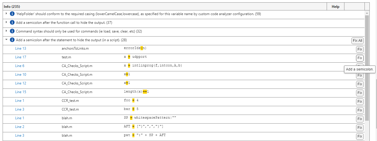
Code Analyzer app with a Fix button

dictionary Object: Access and assign dictionary cell values with curly braces

Data in cells can be looked up and assigned directly using curly braces, {}. When dictionary values are cells, a lookup using parentheses, (), returns a cell. Accessing the contents of that cell requires indexing into the cell. This feature allows contents of cell values to be accessed directly. For example, the dictionary d has three cell values.

d =  

  dictionary (double ⟼ cell) with 3 entries: 

    1 ⟼ {["Hello"]}
    2 ⟼ {[4 5 6]} 
    3 ⟼ {@sin} 

Perform a lookup using parentheses. The lookup returns the value as a cell containing an array.

d(2)
ans =

  1×1 cell array

    {[4 5 6]}

Perform a lookup using curly braces. The lookup returns the value as an array.

d{2}
ans =
    [4 5 6]

Output Argument Validation: Debug within output argument blocks

You can now use the MATLAB debugger within output arguments blocks of functions. While debugging an arguments block, the workspace is read-only. For more information on using the debugger, see Debug MATLAB Code Files.

 Functionality being removed or changed

Warning about indexing with no subscripts (MATLAB:subscripting:noSubscriptsSpecified) has been removed

The warning about indexing into a built-in type with no subscripts (MATLAB:subscripting:noSubscriptsSpecified) has been removed. In previous releases, the warning was off by default, but when users opted in, the warning would appear when indexing with no subscripts.

warning("on","MATLAB:subscripting:noSubscriptsSpecified");
x = [1 2 3 4 5];
y = x()
Warning: A value of class "double" was indexed with no subscripts 
specified. Currently the result of this operation is the indexed value 
itself, but in a future release, it will be an error.

y =

     1     2     3     4     5

Starting in R2023a, the behavior of indexing with no subscripts remains the same and does not error, but the warning no longer appears. Using the warning command to turn the warning on or off has no effect.

Defining classes and packages: Using schema.m will not be supported in a future release

Still runs

Support for classes and packages defined using schema.m files will be removed in a future release. Replace existing schema-based classes with classes defined using the classdef keyword.

Data Analysis

pivot Function: Summarize tabular data using pivot table

Perform a pivoting operation on data in a table or timetable by using the pivot function. Specify grouping variables that define variables or rows in the pivoted table using colvars or rowvars.

Optionally define parameters such as the data variable, function to apply to the data variable, and grouping variable binning schemes by specifying name-value arguments.

table and timetable Data Types: Perform calculations directly on tables and timetables without extracting their data

You can now perform calculations directly on tables and timetables without extracting their data. All the variables in your tables and timetables must have data types that support calculations. You can also perform operations where one operand is a table or timetable and the other is a numeric or logical array. Previously, all calculations required you to extract data from your tables and timetables by indexing into them.

For more information, see Direct Calculations on Tables and Timetables and Rules for Table and Timetable Mathematics.

Timetable Events: Find and label events in timetables using attached event tables

To find and label events in a timetable, attach an event table to it. An event table is a timetable of events. An event consists of an event time (when something happened), often an event length or event end time (how long it happened), often an event label (what happened), and sometimes additional information about the event. Event tables are designed to be attached to timetables. When you attach an event table to a timetable, you can find or label rows in the timetable that occur during events.

MATLAB provides these functions to create event tables from input data, filter timetable rows on event times, and synchronize events to timetables:

combinations Function: Generate all element combinations of arrays

Generate all element combinations of arrays of varying sizes and data types by using the combinations function. Each row of the output table is a combination. Applying the combinations function is equivalent to finding the Cartesian product of sets of elements.

fillmissing2 Function: Fill missing entries in two-dimensional data

Fill missing entries in two-dimensional data sets using the fillmissing2 function. You can fill missing entries using interpolation or moving window methods.

fillmissing Function: Use values from nearest neighbors to fill missing data

You can use the 'knn' method of the fillmissing function to fill missing entries in your data with the corresponding values in the nearest row, based on the pairwise Euclidean distance between rows. You can optionally specify a value k for the 'knn' method to fill missing entries with the mean of the corresponding values in the k nearest rows.

You can also specify a distance function, using the Distance name-value argument, to measure the distance between rows with a specified metric. Distance can have any of these values:

  • 'euclidean' — Euclidean distance (default)

  • 'seuclidean' — Scaled Euclidean distance

  • A function handle — User-specified distance function

Descriptive Statistics and Arithmetic: Omit or include missing data of multiple data types

When analyzing and preprocessing data, you can optionally specify to omit or include numeric, datetime, duration, and categorical missing data. Use the "omitmissing" or "includemissing" flags in addition to any previously supported missing condition flags for these functions:

 Find and Remove Trends Live Editor Task: Interactively find and remove periodic and polynomial trends

The Find and Remove Trends task in the Live Editor can now identify periodic trends for regularly spaced input data. Select the Periodic trend type, and choose the SSA or STL algorithm.

The task can also return polynomial and periodic trends, in addition to the detrended data. Specify Output as Trends.

Previously, this task identified only polynomial trends and returned only the detrended data.

 Compatibility Considerations

To reflect the enhanced functionality of finding and removing periodic and polynomial trends, this task in the Live Editor is now named Find and Remove Trends. Previously, this task was named Remove Trends.

Data Cleaner App: Save session as MAT-file and reload session

When working in the Data Cleaner app, save the session as a binary MAT-file containing the data and cleaning steps. To save the session file, in the File section of the Home tab, click Save. To reload the session, in the File section of the Home tab, click Open.

head and tail Functions: Get top or bottom rows of array

Display or return the top rows of a vector, matrix, multidimensional array, or cell array using the head function, or the bottom rows using the tail function. Previously, head and tail supported only table, timetable, and tall array input data.

 groupsummary Function: Compute number of unique elements

Compute the number of distinct nonmissing elements in each group of data. Specify the "numunique" or "all" method of the groupsummary function, or select the Number of unique values or Select all computation method in the Compute by Group task in the Live Editor.

 Compatibility Considerations

The "all" computation method now returns the number of unique values in addition to the computation methods in the previous release.

 movevars Function: Move table variables after last variable without After name-value argument

When using the movevars function, you can now move variables after the last variable without specifying the After name-value argument.

For example, create a table. Then move the first variable after the last variable.

T = table([1;3;5],[2;4;6],[3;6;9])
T =
  3×3 table
    Var1    Var2    Var3
    ____    ____    ____
     1       2       3  
     3       4       6  
     5       6       9  
T = movevars(T,"Var1")
T =
  3×3 table
    Var2    Var3    Var1
    ____    ____    ____
     2       3       1  
     4       6       3  
     6       9       5  
 Compatibility Considerations

In previous releases, calling movevars without specifying either the After or Before name-value argument resulted in an error. Moving a variable after the last variable required one of these two syntaxes.

T = movevars(T,"Var1","After",width(T))
% or
T = movevars(T,"Var1","After","Var3")

rowfun and varfun Functions: OutputFormat name-value argument can take "auto" as value

The OutputFormat name-value argument can take "auto" as a value. This value is the default value. It causes the rowfun and varfun functions to return outputs whose data types match the data types of their inputs.

day Function: Return ISO day of week

To return the ISO day of week number, use the "iso-dayofweek" option with the day function. In the ISO 8601 standard, Monday is day 1 of the week.

For example, return the ISO day of week number for today.

D = datetime("today");
dayNumber = day(D,"iso-dayofweek")

week Function: Return ISO week of year or week of month

To return the ISO week of year number, use the "iso-weekofyear" option with the week function. In the ISO 8601 standard, a week begins on Monday. Week 1 of a year is defined as the first week in the year with at least four days.

To return the week of month number, use the "iso-weekofmonth" option with the week function. A week begins on Monday. Week 1 of a month is defined as the first week in the month with at least four days. ISO 8601 does not specifically define the week of month number. However, this option returns a week of month number that is consistent with the ISO week of year number.

For example, return the ISO week of year and week of month numbers for today.

D = datetime("today");
weekOfYear = week(D,"iso-weekofyear")
weekOfMonth = week(D,"iso-weekofmonth")

Variables Editor: Edit categories of categorical table variable in MATLAB Online

In the MATLAB Online Variables editor, you can create, remove, or merge categories in a categorical table or timetable variable. To edit the categories, pause on the header of a categorical variable and click the triangle icon, or right-click the variable, and select Edit Categories.

Data Import and Export

Import Data Live Editor Task: Import data in live scripts

The Import Data Live Editor task allows you to import various types of data in a live script within a single framework. You can import these types of data:

  • MAT-file (for example, .mat)

  • Text (for example, .csv)

  • Spreadsheet (for example, .xlsx)

  • Image (for example, .png)

  • Audio (for example, .wav)

  • Video (for example, .avi)

To add the task to a live script in the Live Editor, click Task on the Live Editor tab and select the Import Data icon.

audiowrite Function: Write MP3 audio files

You can write MP3 audio files using the audiowrite function.

imfinfo Function: Get information about XMP metadata embedded in JPEG files

The imfinfo function returns Extensible Metadata Platform (XMP) metadata embedded in JPEG files in the 'XMPData' field of the output structure. The function also returns International Press Telecommunications Council (IPTC) metadata embedded in the XMP namespace. The IPTC data is stored in the 'Iptc4xmpCore' (core metadata) and 'Iptc4xmpExt' (extension metadata) subfields of 'XMPData'.

Parallel Processing: Use readtable in thread-based environments

You can use the readtable function in thread-based environments. Parallel processing results in improved performance when reading data, especially with remote data.

Scientific File Format Libraries: CDF library upgraded to version 3.8.1

The CDF library is upgraded to version 3.8.1.

Scientific File Format Libraries: CFITSIO library upgraded to version 4.1.0

The CFITSIO library is upgraded to version 4.1.0.

 Functionality being removed or changed

web function will return handle to most recent MATLAB web browser as MATLAB class

Behavior change in future release

In a future release, the web function will return a handle to the most recent MATLAB web browser as a MATLAB class. Currently, the web function returns the handle as a Java class. With this change, some methods that were previously supported in the returned handle will no longer be supported.

In most cases, you will not need to make any changes to your code. However, if you are using methods that are not supported in the returned MATLAB class, you will need to update your code.

Mathematics

MATLAB Support Package for Quantum Computing: Build, simulate, and run quantum algorithms

The MATLAB Support Package for Quantum Computing enables you to:

See Quantum Computing and Introduction to Quantum Computing for more information.

To install the MATLAB Support Package for Quantum Computing, locate the support package in Add-On Explorer using the instructions in Get and Manage Add-Ons.

pageeig Function: Perform eigenvalue decomposition on pages of N-D arrays

Use the pageeig function to calculate eigenvalues and eigenvectors of the pages of N-D arrays. In this context, the N-D array is treated as a container for several 2-D matrices.

randi Function: Create random logical array

Use randi to create a random logical array by specifying the typename argument as "logical" or the prototype p as a logical array.

For example, you can create a 5-by-5 random logical array using randi([0 1],5,"logical").

 Functionality being removed or changed

spy plots have adjusted default behavior for aspect ratio and marker size

Behavior change

The aspect ratio of spy plots has a 1-to-10 limit, after which the plot stops adjusting to the matrix shape. You can use pbaspect("auto") for no special aspect ratio or pbaspect([size(A,2) size(A,1) 1]) for the previous behavior of a matching aspect ratio, even for very "squeezed" cases.

Additionally, the default marker size is based only on the matrix size. Previously, the point size of the axes on creation could also affect the marker size.

Graphics

xregion and yregion Functions: Highlight horizontal or vertical regions of plots

Highlight one or more horizontal or vertical regions of a plot with the xregion and yregion functions. You can set properties to customize the color and boundary lines of these shaded regions.

Two charts with highlighted regions. The bar chart has a shaded horizontal region. The line plot has a shaded vertical region.

sky Function: Apply monochromatic colormap to charts

Use the sky function to color charts with the same monochromatic colormap that heatmap charts use. Like for all predefined colormaps, you can optionally specify the number of colors for the sky colormap.
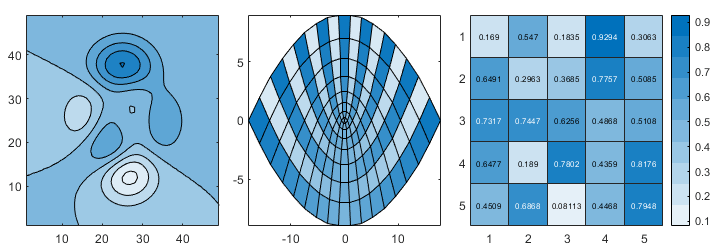
Three charts that use the sky colormap

tiledlayout Function: Create horizontal or vertical layouts

Create horizontal or vertical layouts by specifying "horizontal" or "vertical" as the first input argument to the tiledlayout function. For example, create a horizontal layout and add three plots.

tiledlayout("horizontal")
x = 1:5;
nexttile
plot(x)
nexttile
bar(x);
nexttile
contourf(peaks)
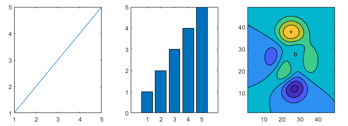
Three plots in a horizontal layout

animatedline Function: Create animated lines using numeric, datetime, or duration data

Use the animatedline function to create animated lines using single, double, integer, datetime, or duration data for the x-, y-, and z-coordinates.

Grid Lines: Customize grid line thickness

Change the thickness of grid lines independently of the box outline and tick marks by setting the GridLineWidth and MinorGridLineWidth properties of the axes. Before R2023a, the LineWidth property of the axes was the only property for controlling the grid line width. However, that property controlled the grid lines, box outline, and tick marks together. Now you can control the thickness of the grid lines separately.
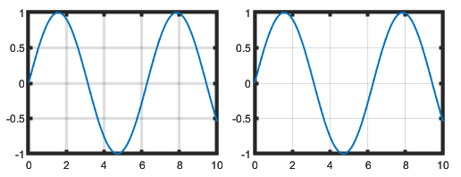
Two line plots with the same box outline and tick mark thickness, but with different grid line thicknesses

Axes Labels: Rotate x- and y-axes labels without overlapping the axes

When you change the Rotation property of an axis label in a 2-D plot, the HorizontalAlignment and VerticalAlignment properties of the label automatically change to prevent overlap between the label and the axes.

For example, create a plot with a y-axis label.

plot([0 3 1 6 4 10])
ylab = ylabel("Y Data");
Line plot that has a y-axis label with words flowing from bottom to top

Rotate the label so that the text is horizontal. MATLAB automatically adjusts the HorizontalAlignment and VerticalAlignment properties to prevent the overlap.

ylab.Rotation = 0;
Line plot that has a y-axis label with words flowing from left to right

Plotting Series of Lines: Control cycling order of line styles

When plotting a series of multiple lines, you can use the LineStyleCyclingMethod property of the axes to control how different lines are distinguished from one another. Specify this property as one of these values:

  • "withcolor" — Cycle through the line styles with the colors

  • "beforecolor" — Cycle through the line styles before cycling through the colors

  • "aftercolor" — Cycle through the line styles after cycling through the colors (default)
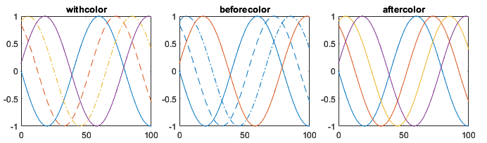
Three axes that each contain four plotted lines with different line style cycling methods

Plotting Series of Lines: Control whether the data range of a line affects automatic axes limits

Specify whether a specific line affects the automatically selected axes limits by setting the AffectAutoLimits property. By default, the axes limits change to encompass the data range for each successive line you create. Setting this property enables you to focus on the range of a subset of lines in the axes.

Two line plots, each showing the same two data sets as a thin red line and thick blue line, but with different x-axis limits. The x-values of the thin red line range from –100 to 100. The x-values of the thick blue line range from 0 to 100. The x-axis in the left plot spans the range [–100, 100]. The x-axis in the right plot spans the range [0, 100]. As a result, the right plot excludes part of the thin red line.

fontsize and fontname Functions: Optionally specify the object containing the text

When calling the fontsize or fontname functions, you can omit the object argument when you want the functions to affect the current figure.

DatetimeRuler Object: Set or get the reference date for plotting datetime values

Set the ReferenceDate property of a DatetimeRuler object when you plot datetime values. This property is useful for synchronizing tick placement across different axes and for plotting data from different time zones together.

Image Display Preferences: Access and update imshow preferences in MATLAB Online

In MATLAB Online, you can set the default values for these aspects of images displayed using imshow:

  • Axes visible — Control whether imshow displays images with the axes box outline and tick labels.

  • Border Style — Control whether imshow draws a tight or loose border around images in the figure window.

  • Initial Magnification — Control whether imshow initially fits images to the figure window or magnifies them by a specified percentage.

To open these image display preferences, on the Home tab, in the Environment section, click Preferences button Preferences. Select MATLAB > Image Display.

 Functionality being removed or changed

BaseValue property of bar, stem, and area plots no longer changes with axes limits

Behavior change

The BaseValue property of bar, stem, and area plots no longer depends on the axes limits. The property value stays the same when you change axes limits or pan within the axes.

This change does not affect the appearance of the plots, but it provides a more predictable experience when you change the axes limits or pan within the axes.

MATLAB Online limits imshow image display resolution

Behavior change

MATLAB Online limits the maximum imshow image display resolution to improve rendering speeds for large images. This behavior affects the on-screen display, but it does not affect the image data. Before displaying an image, imshow resizes the largest dimension to a maximum size of 512 pixels. The smaller dimension adjusts to preserve the aspect ratio of the image. To view images at their full resolution, use MATLAB desktop or set the MaxRenderedResolution property of the output Image object to "none". For details about the MaxRenderedResolution property, see Image Properties.

Plot Catalog tool will be removed

Warns

The Plot Catalog tool will be removed in a future release. Instead, to interactively create and explore visualizations for your data, use the Plots tab in the MATLAB Toolstrip or the Create Plot task in the Live Editor.

For more information about visualizations, see Types of MATLAB Plots or toolbox-specific documentation.

Figure Tools menu will no longer include interaction modes and options

Still runs

In a figure, the Tools menu will no longer contain these items in a future release:

  • Zoom In

  • Zoom Out

  • Pan

  • Rotate 3D

  • Data Tips

  • Brush

  • Restore View

  • Options

  • Align Distribute Tool

Instead, to enable interaction modes, use the axes toolbar. Customize the interaction by right-clicking in the chart when an interaction mode is enabled, or for apps, by using the InteractionOptions property of the axes.

App Building

addStyle Function: Add styles to items in list box or drop-down UI component

Create styles for specific items in a list box or drop-down UI component using the uistyle and addStyle functions. For example, you can add icons to items in a list box. To get information on applied styles, query the StyleConfigurations property of the ListBox or DropDown object. To remove a style from a component, use the removeStyle function.

uistack Function: Change stacking order of UI components in UI figure

You can now use the uistack function to change the stacking order of UI components and containers in a figure created using the uifigure function. Previously, uistack supported UI components only in figures created using the figure function.

uipanel and uibuttongroup Functions: Specify container border color

You can specify the border color of panels and button groups by using the BorderColor property. For more information, see Panel Properties or ButtonGroup Properties.

uihtml Function: Send events between MATLAB and HTML

When you create an HTML UI component using the uihtml function, you can send events between MATLAB and HTML. Send events when a specific action occurs to one object and another object needs to know about or react to that action. For example, you can send an event from HTML to MATLAB whenever a user clicks a button HTML element, and then write a callback in MATLAB that updates your app in response. You also can send an event from MATLAB to HTML whenever a user clicks a Button UI component in your app, and then write a callback in your HTML source file that updates the HTML code in response.

To send an event from HTML to MATLAB, call the sendEventToMATLAB function on the htmlComponent JavaScript® object in your setup method.

htmlComponent.sendEventToMATLAB(eventName,eventData)

React to this event by writing MATLAB code that creates an HTMLEventReceivedFcn callback for the HTML MATLAB object.

comp.HTMLEventReceivedFcn = @myCallbackFunction

To send an event from MATLAB to HTML, call the sendEventToHTMLSource function on the HTML MATLAB object.

sendEventToHTMLSource(comp,eventName,eventData)

React to this event by writing JavaScript code in your setup method that listens for the event and executes a callback function in response.

htmlComponent.addEventListener(eventName,eventData,callbackFunction)

For more information, see Send Event from JavaScript to MATLAB and Send Event from MATLAB to JavaScript.

uiimage Function: Specify image alt text for use with screen readers

Provide a description of an image created using the uiimage function by specifying the AltText property. This property is used by screen readers to describe the image when an app user navigates through the app.

appmigration.migrateGUIDEApp Function: Programmatically migrate existing GUIDE apps to App Designer

Programmatically migrate existing GUIDE apps to App Designer apps by using the appmigration.migrateGUIDEApp function. You can specify a single app, multiple apps, or a folder of apps to migrate as a batch. The function uses the GUIDE to App Designer Migration Tool for MATLAB to perform the migration.

App Designer: View progress when loading an app

When you load an app in App Designer, a progress bar now displays an estimate of its loading progress.
App Designer progress dialog box. The dialog box has text "Opening myApp.mlapp..." and the progress bar shows 48% completion.

App Designer: Add label to unlabeled UI component

To add a label to a UI component without one, in Design View, right-click the component and select Add Label or use the keyboard shortcut Ctrl+L.
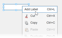
Edit field context menu. The top option is "Add Label".

App Designer: Replace assigned callback with new callback

You can now more efficiently create a new callback for a UI component that already has a callback assigned. To replace an existing callback with a new one, select the component in the Component Browser and, in the Callbacks tab, select the option to add a callback. For example, for a component with a ButtonPushedFcn callback already assigned, select <add ButtonPushedFcn callback> from the associated drop-down list. App Designer creates a new callback function, assigns it to the component, and unassigns the previous callback function.
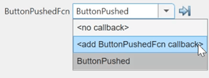
ButtonPushedFcn drop-down list. The second option is "<add ButtonPushedFcn callback>".

Previously, you had to first unassign the assigned callback from the component before creating a new callback.

App Testing Framework: Test context menus within labels

You can use the chooseContextMenu method to test a right-click that opens a context menu within label components. For example, assign a context menu with two items to a label, and then choose the first menu item.

fig = uifigure;
lbl = uilabel(fig);

cm = uicontextmenu(fig);
m1 = uimenu(cm,Text="Menu1");
m2 = uimenu(cm,Text="Menu2");
lbl.ContextMenu = cm;

testCase = matlab.uitest.TestCase.forInteractiveUse;
testCase.chooseContextMenu(lbl,m1)

Axes Interactions: Customize behavior of interactions with axes view

For apps created in App Designer and using the uifigure function, customize axes interaction behavior using the InteractionOptions property of the axes. Customize the behavior of panning, zooming, rotating, adding data tips, data brushing, and restoring the original view by setting the value of InteractionOptions properties. For a complete list of properties, see InteractionOptions Properties.

The options set by the InteractionOptions object apply to these interactions on the associated axes:

  • The built-in interactions specified by the Interactions property of the axes

  • Interactions enabled by using mode functions, such as pan and zoom

  • Interactions enabled using the axes toolbar

For example, limit all pan and zoom interactions to the x-dimension only.

fig = uifigure;
ax = uiaxes(fig);
ax.InteractionOptions.LimitsDimensions = "x";

Plots in Apps: Enable data cursor mode

For apps created in App Designer and using the uifigure function, use data cursor mode to interactively create and edit data tips. For supported charts, select the Data Tips icon in the axes toolbar or use the datacursormode function.

Plots in Apps: Specify axes for interaction mode

For apps created in App Designer and using the uifigure function, set the interaction mode for axes. Specify the Axes object as the first argument for these functions:

For example, for a figure with two axes, enable pan mode for only axes ax1.

fig = uifigure;
t = tiledlayout(fig,1,2);
ax1 = nexttile(t);
ax2 = nexttile(t);
pan(ax1,"on")

When setting the interaction mode for axes, these functions do not return pan, zoom, rotate3d, DataCursorManager, or brush objects. Previously, these functions set the interaction mode for all Axes children of the current or target figure.

 Functionality being removed or changed

uistack function has different stacking behavior for menus, toolbars, push tools, and toggle tools

Behavior change

When you modify the stacking order of menus, toolbars, push tools, and toggle tools using the uistack function, the behavior is different than in previous releases. For example, starting in R2023a, calling uistack(comp,"up") has this behavior:

  • Menu items parented to a figure — The menu item moves one place to the left in the menu bar. Previously, the menu item moved one place to the right.

  • Menu items parented to a context menu — The menu item moves one place up in the context menu. Previously, the menu item moved one place down.

  • Toolbars — The toolbar moves one place up within the collection of toolbars in the figure. Previously, the toolbar moved one place down.

  • Push tools and toggle tools — The push tool or toggle tool moves one place to the left in the toolbar. Previously, the push tool or toggle tool moved one place to the right.

If your code uses uistack to modify the stacking order of menus, toolbars, push tools, or toggle tools, make these updates to the code to retain the previous behavior.

Original Code in R2022b or EarlierUpdated Code in R2023a
uistack(comp,"top")uistack(comp,"bottom")
uistack(comp,"up",step)uistack(comp,"down",step)
uistack(comp,"bottom")uistack(comp,"top")
uistack(comp,"down",step)uistack(comp,"up",step)

HighlightColor property of panel and button group containers is not recommended

Still runs

Using the HighlightColor property to specify the border color of a panel or button group is not recommended. Use the BorderColor property instead. The BorderColor property has the same effect and accepts the same values as the HighlightColor property. For more information, see Panel Properties or ButtonGroup Properties.

There are no plans to remove support for the HighlightColor property at this time. However, the HighlightColor property no longer appears in the list returned by calling the get function on a UI container.

Performance

Language and Programming: Improved performance when calling functions and methods

Calling most functions and methods shows improved performance. For example, in a file named myFun.m in your current folder, create the myFun function.

function y = myFun(x)
y = x;
end

In a file named timingTest.m in your current folder, create a function that calls myFun. The timingTest function is about 1.6x faster than in the previous release.

function out = timingTest
n = 1e7;
for i = 1:n
    out = myFun(3);
end
end

The approximate execution times are:

R2022b: 0.18 s

R2023a: 0.11 s

The code was timed on a Windows 10, Intel Xeon CPU E5-1650 v4 @ 3.60 GHz test system using the timeit function.

timeit(@timingTest)

Function Handles: Improved performance when invoking handles to named functions

Invoking handles to named functions that are not nested shows improved performance. Invoking such function handles no longer results in an overhead compared to calling functions directly. For example, in a file named myFun.m in your current folder, create the myFun function.

function y = myFun(x)
y = x;
end

In a file named timingTest.m in your current folder, create a function that invokes a handle to myFun. The timingTest function is about 40x faster than in the previous release.

function t = timingTest
f = @myFun;
n = 1e7;
tic
for i = 1:n
    out = f(3);
end
t = toc;
end

The approximate execution times are:

R2022b: 4.4 s

R2023a: 0.11 s

The code was timed on a Windows 10, Intel Xeon CPU E5-1650 v4 @ 3.60 GHz test system by calling the timingTest function.

varargin Argument: Improved performance when specifying zero or more inputs

Specifying a variable number of input arguments using varargin shows improved performance. For example, in a file named timingTest.m in your current folder, create a function that expects one input and accepts an additional number of inputs.

function timingTest(x,varargin)
n = 1e6;
tic
for i = 1:n
    y = myFun(x,varargin{:});
end
toc
end

function y = myFun(x,varargin)
if nargin == 1
    y = x;
elseif nargin == 3
    y = x + varargin{1} + varargin{2};
else
    y = NaN;
end
end

The amount of improvement depends on whether varargin is empty. The performance improvement is most significant when varargin is empty.

  • Empty varargin — Time this code by running timingTest(1). The code is about 22x faster than in the previous release. The approximate execution times are:

    R2022b: 0.404 s

    R2023a: 0.018 s

  • Nonempty varargin — Time this code by running timingTest(1,2,3). The code is about 2x faster than in the previous release. The approximate execution times are:

    R2022b: 1.428 s

    R2023a: 0.734 s

The code was timed on a Windows 10, Intel Xeon CPU E5-1650 v4 @ 3.60 GHz test system.

timetable Data Type Indexing: Improved performance when subscripting with times or with withtol subscript

timetable subscripting when subscripting with times or with a withtol subscript is significantly faster in R2023a than in R2022b.

  • For example, when you use a vector of 100 datetime values to subscript into a timetable that has 107 rows, performance in R2023a is about 114x faster than in R2022b.

    function timingTest()
    rng default
    
    % 10^7 rows
    N = 10000000;
    rowtimes = datetime(2023,1,1,0,0,0:N-1); 
    rowtimes.Format = rowtimes.Format + ".SSS";
    tt = timetable(rand(N,1),RowTimes=rowtimes);
    
    % 100 values chosen in steps of 10
    n = 1000;
    t = datetime(2023,1,1,0,0,0:10:n-1);
        
    tic
    tt2 = tt(t,:);
    toc
    end
    

    The approximate execution times are:

    R2022b: 9.10 s

    R2023a: 0.08 s

  • Similarly, when you use a vector of 100 duration values to subscript into a timetable that has 107 rows, performance in R2023a is about 14x faster than in R2022b.

    function timingTest()
    rng default
    
    % 10^7 rows
    N = 10000000;
    rowtimes = seconds(0:N-1);
    tt = timetable(rand(N,1),RowTimes=rowtimes);
    
    % 100 values chosen in steps of 10
    n = 1000;
    t = seconds(0:10:n-1);
        
    tic
    tt2 = tt(t,:);
    toc
    end
    

    The approximate execution times are:

    R2022b: 1.29 s

    R2023a: 0.09 s

  • When you use a withtol subscript with a timetable that has 107 rows, performance in R2023a is about 44x faster than in R2022b.

    function timingTest()
    rng default
    
    % 10^7 rows
    N = 10000000;
    rowtimes = seconds(0:N-1);
    tt = timetable(rand(N,1),RowTimes=rowtimes);
    
    % 100 values chosen in steps of 10
    n = 1000;
    t = seconds(0:10:n-1);
    
    tt.Time = tt.Time + .1*seconds(rand(N,1));
    wt = withtol(t,seconds(.1));
        
    tic
    tt2 = tt(wt,:);
    toc
    end
    

    The approximate execution times are:

    R2022b: 3.92 s

    R2023a: 0.09 s

The code was timed on a Windows 10, AMD EPYC 74F3 24-Core Processor @ 3.19 GHz test system by calling each version of the timingTest function.

Complex Matrices: Improved performance when using colon indexing to copy complex matrices

Copying a complex matrix using colon indexing shows improved performance. This improvement is greater for larger matrices.

For example, this code is about 105x faster than in the previous release.

a = rand(100)*1j; 

tic; 
for i = 1:1e6 
    b = a(:,:); 
end 
toc; 

The approximate execution times are:

R2022b: 22.3 s

R2023a: 0.212 s

This improvement is most noticeable when the copy is not modified. However, examples like these still execute noticeably faster.

  • Modify no elements of the copy based on a conditional (95x improvement).

    a = rand(100)*1j; 
    
    tic; 
    for k = 1:1e6
        b = a(:,:);
        if (isreal(b(1,1)))
            b(1,1) = b(1,1)*1j;
    end 
    toc;
    

    R2022b: 21.3 s

    R2023a: 0.223 s

  • Modify an element of the copy based on a conditional (2x improvement).

    a = rand(100)*1j; 
    
    tic; 
    for k = 1:1e6
        b = a(:,:);
        if (~isreal(b(1,1)))
           b(1,1) = b(1,1)*1j;
    end 
    toc;
    

    R2022b: 23.5 s

    R2023a: 10.1 s

  • Use an implicit copy in an operation (4x improvement).

    a = rand(100)*1j;
    b = rand(100)*1j;
    
    tic;
    for k = 1:1e6
        c = a(:,:) + b;
    end
    toc;
    

    R2022b: 41.1 s

    R2023a: 9.87 s

  • Resize from 4-D to 2-D during copy (63x improvement).

    a = rand(10,10,10,10)*1j;
    
    tic;
    for k = 1:1e6
        b = a(:,:);
    end
    toc;
    

    R2022b: 28.2 s

    R2023a: 0.451 s

The code was timed on a Windows 10, Intel Xeon CPU E5-2650 v2 @ 2.60 GHz test system.

mean, std, var, and rmse Functions: Improved performance when computing along default vector dimension

The mean, std, var, and rmse functions show improved performance when computing over a real vector when the operating dimension is not specified. The functions determine the default operating dimension more quickly in R2023a than in R2022b.

For example, this code computes the mean along the default vector dimension. The code is about 2.2x faster than in the previous release.

function timingMean
A = rand(10,1);
for i = 1:8e5
    mean(A);
end
end

The approximate execution times are:

R2022b: 0.91 s

R2023a: 0.41 s

The code was timed on a Windows 10, Intel Xeon CPU E5-1650 v4 @ 3.60 GHz test system using the timeit function.

timeit(@timingMean)

Moving Statistics Functions: Improved performance when computing over matrix with sample points

Moving statistics functions show improved performance when computing over a matrix when there are sample points. These functions show improved performance:

For example, this code computes the moving sums of a 300-by-300 matrix with corresponding sample points. The code is about 3x faster than in the previous release.

function timingMovsum
A = randn(300);
t = sort(rand(300,1));
tic
for k = 1:2000
    movsum(A,0.1,"SamplePoints",t);
end
toc
end

The approximate execution times are:

R2022b: 1.04 s

R2023a: 0.34 s

The code was timed on a Windows 10, Intel Xeon CPU E5-1650 v4 @ 3.60 GHz test system by calling the timingMovsum function.

histcounts Function: Improved performance with small numeric and logical input data

The histcounts function shows improved performance for numeric and logical data due to faster input parsing. The performance improvement is more significant when input parsing is a greater portion of the computation time. This situation occurs when the size of the data to distribute among bins is smaller than 2000 elements.

For example, this code calculates histogram bin counts for a 1000-element vector. The code is about 3x faster than in the previous release.

function timingHistcounts
X = rand(1,1000);
for k = 1:3e3
    histcounts(X,"BinMethod","auto");
end
end

The approximate execution times are:

R2022b: 0.62 s

R2023a: 0.21 s

The code was timed on a Windows 10, Intel Xeon CPU E5-1650 v4 @ 3.60 GHz test system using the timeit function.

timeit(@timingHistcounts)

fzero function: Improved performance

The fzero function shows improved performance. The performance improvement is most significant when the objective function is fast to compute and fzero does not use an options argument.

For example, this code runs about 4x faster than in the previous release.

rng default
N = 1e5;
levels = 1.5 * rand(N,1);
out = zeros(N,1);
myfun = @(x,lv)x*sin(x)-lv;
tic
for i=1:N
    out(i) = fzero(@(x)myfun(x,levels(i)),0);
end
toc

The approximate execution times are:

R2022b: 2.67 s

R2023a: 0.63 s

The code was timed on a Windows 10, Intel Xeon CPU E5-1650 v3 @ 3.5 GHz test system.

Plots in Apps: Improved performance when rerendering axes

Axes rerender more quickly in R2023a than in R2022b. The reduced rerendering time is most noticeable when many sequential updates to the axes occur.

For example, first create axes to specify as the input to the timingAnimation function. Then, call the timingAnimation function to add points to an animated line. The time for the axes to rerender is reduced, resulting in an animation that is about 1.35x faster in R2023a than in the previous release.

function timingAnimation(ax)
h = animatedline(ax);
x = linspace(0,4*pi,1000);
y = sin(x);
tic
for k = 1:length(x)
    addpoints(h,x(k),y(k));
    drawnow
end
toc
end

The approximate durations of the animation are:

R2022b: 5.66 s

R2023a: 4.20 s

The code was timed on a Windows 10, Intel Xeon CPU E5-1650 v4 @ 3.60 GHz test system by calling the timingAnimation function.

Plots in Apps: Improved performance when creating axes

Axes render more quickly within apps and within figures created with the uifigure function in R2023a than in R2022b. The delay before the axes appear in an existing figure is reduced.

For example, if you run the code uiaxes(f) for an existing figure f, the axes appear about 3.7x faster in R2023a than in R2022b when creating axes for the first time in a MATLAB session and about 2.4x faster for subsequent axes.

The approximate axes rendering times are:

 First AxesSubsequent Axes
R2022b14.94 s1.06 s
R2023a4.02 s0.44 s

These operations were timed on a Windows 10, Intel Xeon CPU E5-1650 v4 @ 3.60 GHz test system.

Plots in Apps: Improved responsiveness of ruler-pan interaction

The ruler-pan interaction is faster and smoother within apps and within figures created with the uifigure function in R2023a than in R2022b. The improvement is most noticeable for plots that display a large number of data points.

For example, this code creates a figure with a plot of a 2500-by-2500 matrix. When you pan the ruler, the ruler-pan interaction is smoother and the axes track your mouse motion more closely in R2023a than in the previous release.

f = uifigure;
ax = uiaxes(f);
p = peaks(2500);
plot(ax,p)

R2022bR2023a

When panning the ruler, the surface plot takes a moment to reposition and jumps to the new location.

Animation of panning the y-axis ruler of a surface plot in R2022b

When panning the ruler, the surface plot follows the mouse motion more closely and repositions more quickly at the new location.

Animation of panning the y-axis ruler of a surface plot in R2023a

The ruler-pan interaction was performed on a Windows 10, Intel Xeon CPU E5-1650 v4 @ 3.60 GHz test system by running the above script and panning the y-axis ruler.

Live Editor: Improved performance when filtering numeric table variables

In the output of the Live Editor, the performance of filtering a numeric table or timetable variable is improved. When dragging the maximum or minimum value slider, the drag interaction is smoother and faster in R2023a than in R2022b, and the data tip displaying the current slider value appears to the side of the filtering figure.

For example, for a table output in the Live Editor, pause on the header of a numeric variable and click the triangle icon. Then, to filter the data, adjust the maximum value by dragging the slider. The drag interaction is smoother and tracks your mouse motion more closely in R2023a than in the previous release.

R2022bR2023a

After dragging the maximum value slider in a filtering figure, the slider takes a moment to reposition and jumps to the new location. The associated data tip moves with the slider and obscures the filtering figure.

Animation of dragging the slider in a filtering figure in R2022b

After dragging the maximum value slider in a filtering figure, the slider follows the mouse motion more closely and repositions more quickly at the new location. The associated data tip is located in a fixed position to the right of the filtering figure.

Animation of dragging the slider in a filtering figure in R2023a

The filtering interaction was performed on a Windows 10, Intel Xeon CPU E5-1650 v4 @ 3.60 GHz test system by dragging the maximum value slider in the filtering figure for a 1000-row numeric table variable.

Property Inspector: Improved performance when opening for the first time

The Property Inspector shows improved performance when opening for the first time in a MATLAB session. The delay between clicking the Property Inspector icon or calling inspect and the inspector being ready is reduced.

For example, open the Property Inspector for the first time in a MATLAB session. You can use the Property Inspector 1.17x sooner than in the previous release.

ax = axes;
inspect(ax)

The approximate rendering times are:

R2022b: 13.5 s

R2023a: 11.5 s

The rendering of the Property Inspector was timed on a Windows 10, Intel Xeon CPU E5-1650 v4 @ 3.60 GHz test system by running the code and measuring the time it takes for the edit fields to appear in the Property Inspector.

Property Inspector: Improved performance when switching between objects

The Property Inspector shows improved performance when switching between objects. The delay between selecting a different object and an existing instance of the Property Inspector rendering the properties of the newly selected object is reduced.

For example, open the Property Inspector. Then, create and inspect an Axes object. The axes properties render 1.7x faster than in the previous release.

inspect
ax = axes;
inspect(ax)

The approximate times for the Property Inspector to render the properties of the axes are:

R2022b: 3.5 s

R2023a: 2.1 s

The rendering of the Property Inspector was timed on a Windows 10, Intel Xeon CPU E5-1650 v4 @ 3.60 GHz test system by running the code and measuring the time it takes for the Property Inspector to be ready.

Variables Editor: Improved performance of cell editing in MATLAB Online

In the MATLAB Online Variables editor, when you interactively edit the value of a cell, the cell updates to display the new value more quickly in R2023a than in R2022b.

For example, create a 1000-element cell array and open the cell array in the Variables editor.

C = cell(1000);
openvar C

Then, double-click on a cell and enter a new value. On a Windows 10, Intel Xeon CPU E5-1650 v4 @ 3.60 GHz test system, when you move the focus from the edited cell, the cell value updates immediately. In R2022b, the cell value updates after a 3.5-second delay.

Variables Editor: Improved speed of data display when scrolling in MATLAB Online

In the MATLAB Online Variables editor, the performance of vertical and horizontal scrolling is improved. When scrolling within 1000 rows below the current element or 100 variables to the right of the current element, the data appears more quickly in R2023a than in R2022b.

For example, create a 1000-by-1000 matrix and open the matrix in the Variables editor.

X = rand(1000);
openvar X

When you scroll down 100 rows, the values of all visible matrix elements in the Variables editor are rendered about 6.7x faster than in the previous release.

The approximate times for the Variables editor to render the values of all visible matrix elements are:

R2022b: 1.80 s

R2023a: 0.27 s

This interaction was timed on a Windows 10, Intel Xeon CPU E5-1650 v4 @ 3.60 GHz test system by running the above script and scrolling in the Variables editor.

App Building: Improved app startup performance

Apps created in App Designer and using the uifigure function start up faster in R2023a than in R2022b and previous releases. The improvement is more noticeable for apps with many UI components.

For example, this code creates an app with 1000 edit field components. The code is about 1.5x faster than in the previous release and about 3x faster than in R2021b.

function timingApp
fig = uifigure;
gl = uigridlayout(fig,Scrollable="on");
gl.RowHeight = repmat({'fit'},1,100);
gl.ColumnWidth = repmat({'fit'},1,10);

for k = 1:1000
    uieditfield(gl);
end
end

The approximate execution times are:

R2021b: 21.5 s

R2022b: 10.6 s

R2023a: 7.2 s

The code was timed on a Windows 10, Intel Xeon CPU E5-1650 v4 @ 3.60 GHz test system by running the timingApp function and measuring the time it takes for the edit fields to appear in the UI figure window.

 App Building: Improved startup performance for apps with multiple tabs

In addition to the overall app startup performance improvement in R2023a, some apps that contain multiple tabs show an even greater startup performance improvement. The reason is that MATLAB prioritizes creating the content in the visible tab over non-visible content when the app first runs.

The particular performance improvement that you see depends on the app layout and UI component types. The improvement is more noticeable for apps with these types of UI components in unselected tabs:

  • Labels and spinners with a grid layout manager

  • Table UI components without a grid layout manager

For example, this code creates a tab group with five tabs, each containing 200 label components. The code is about 1.9x faster than in the previous release.

function timingTabApp
fig = uifigure;
tg = uitabgroup(fig);

for k1 = 1:5
    t = uitab(tg);
    gl = uigridlayout(t,Scrollable="on");
    gl.RowHeight = repmat({'fit'},1,20);
    gl.ColumnWidth = repmat({'fit'},1,10);
    for k2 = 1:200
        uilabel(gl);
    end
end
end

The approximate execution times are:

R2022b: 9.8 s

R2023a: 5.2 s

The code was timed on a Windows 10, Intel Xeon CPU E5-1650 v4 @ 3.60 GHz test system by running the timingTabApp function and measuring the time it takes for the components to appear in the UI figure window.

If you have an app with many UI components, consider updating your app layout to take advantage of this improvement. For more information, see Improve App Startup Time.

 Compatibility Considerations

When an app user switches to a new tab for the first time after running an app, the interaction might take more time than in previous releases. The reason is that MATLAB might create some content in the tab only after the user selects the tab. If the user later switches to the same tab again, the interaction does not take the additional time.

App Building: Improved performance when resizing some apps

When a user resizes an app figure window, some apps reposition their content faster in R2023a than in R2022b. The types of apps that show this improvement are:

  • Large apps with tabs that have an AutoResizeChildren value of 'on'

  • Large apps with panels and button groups that have a SizeChangedFcn callback

For example, this code creates an app with a tab group where each tab contains many edit fields that are resized automatically. The resize operation is smoother and faster in R2023a than in the previous release.

function tabResize
fig = uifigure;
tg = uitabgroup(fig,"Position",[20 20 400 375]);
for k1 = 1:5
    t = uitab(tg,"Scrollable","on");
    for k2 = 1:100
        ef = uieditfield(t,"Position",[50 22*k2 250 20]);
    end
end
end
R2022bR2023a

When the app resizes, the app content takes multiple seconds to reposition.

When the app resizes, the app content takes less than one second to reposition.

As another example, this code creates an app with many panels, each of which resizes a button using a SizeChangedFcn callback whenever the app size changes. The resize operation is smoother and faster in R2023a than in the previous release.

function panelResize
fig = uifigure("AutoResizeChildren","off", ...
    "SizeChangedFcn",@resizePanels);
for k = 1:225
    p = uipanel(fig, ...
        "AutoResizeChildren","off", ...
        "SizeChangedFcn",@resizeButtons);
    btn = uibutton(p,"Position",[2 2 20 20]);
end
end
 
function resizeButtons(src,~)
for k = 1:length(src.Children)
    src.Children(k).Position(3:4) = 0.9*src.Position(3:4);
end
end

function resizePanels(src,~)
xscale = src.Position(3)/15;
yscale = src.Position(4)/15;
for k = 1:length(src.Children)
    p = src.Children(k);
    p.Position = [xscale*(mod((k-1),15)), ...
        yscale*(floor((k-1)/15)), ...
        xscale, ...
        yscale];
end
end
R2022bR2023a

When the app resizes, the app content takes multiple seconds to reposition.

Animation of resizing a figure window with many panels that each contain a button in R2022b

When the app resizes, the app content takes about one second to reposition.

Animation of resizing a figure window with many panels that each contain a button in R2023a

The resize interactions were performed on a Windows 10, Intel Xeon CPU E5-1650 v4 @ 3.60 GHz test system by running the tabResize and panelResize functions and resizing the figure window.

Software Development Tools

Build Automation: Improve build speed and efficiency with incremental builds

The build tool supports incremental builds. Incremental builds avoid redundant work by skipping tasks that are up to date. If you want the build tool to skip a task when it is up to date, specify the inputs or outputs of the task. The build tool keeps track of the inputs and outputs every time the task runs and skips the task if they have not changed. For more information, see Improve Performance with Incremental Builds.

Build Automation: Create and run tasks that accept arguments

The build tool lets you create and run tasks that accept arguments. You can use task arguments to customize the actions that tasks perform when they run. For more information, see Create and Run Tasks That Accept Arguments.

Dependency Analyzer: Analyze files and folders with or without a project

Starting in R2023a, you can access Dependency Analyzer from the MATLAB apps gallery. You can now perform a dependency analysis on files and folders that do not belong to a project. For more information, see Dependency Analyzer.

Project Preferences: Recreate empty project folders in Git repositories

Git does not track empty folders and ignores them when you commit. MATLAB now enables you to recreate an empty folder structure in a project under Git source control. Doing so is useful for small projects intended for training or as procedure templates.

For large projects, to avoid performance issues on startup, clear Recreate empty project folders in a project under Git. For more information, see Set MATLAB Projects Preferences.

Project API: Determine if file is under project root folder

You can now programmatically determine whether a file or a folder is under a project root folder by using the matlab.project.isUnderProjectRoot function.

Project API: Export subset of project files to archive

You can now programmatically export a subset of project files to an archive by specifying a user-defined export profile in the export function.

Project Sharing: Include only specific files in project archive using export profile

You can now use an export profile to include only files with particular labels in a project archive. This option is useful if the files you need to share are only a small subset of a large project. For more information, see Create an Export Profile.

Comparison Tool: Automate comparison report generation for continuous integration (CI) workflows

Starting in R2023a, you can programmatically publish comparison reports for plain text files, MATLAB scripts, and text-based source code files. Automate report generation for continuous integration (CI) workflows using the visdiff function.

comparison = visdiff(textfile1,textfile2);
file = publish(comparison);
web(file)

Source Control in MATLAB Online: Save uncommitted changes by creating a Git stash

In MATLAB Online, you can now save uncommitted changes by creating a Git stash.

Source Control in MATLAB Online: Manage Git remote repositories locally using Branch Manager

In MATLAB Online, you can now manage multiple remote repositories from a local Git repository. Use Branch Manager to perform these tasks:

  • Add, edit, and delete remote repositories.

  • Fetch from all remotes or individual remotes.

  • Prune remote branches from all or individual remotes.

  • Open selected remotes in a web browser.

  • Create new local branches that track remote branches.

  • Delete remote branches.

Source Control in MATLAB Online: Detect and extract conflict markers from text and binary files

In MATLAB Online, you can now detect conflict markers added by Git in text and binary files. Extract conflict markers to repair corrupted files.

Comparison Tool in MATLAB Online: Compare project definition files

Starting in R2023a, when you compare folders in MATLAB Online, MATLAB detects whether they are project root folders. MATLAB looks for and compares the project definition files stored in the resources or .SimulinkProject folder. Project definition files contain information about the project path, project settings, shortcuts, labels, and referenced projects. For more information, see Compare MATLAB Projects in MATLAB Online.

Dependency Analyzer in MATLAB Online: Investigate circular dependencies using the Project Hierarchy view

You can now investigate how projects in your hierarchy relate to each other and identify projects that introduce circular dependencies using the Project Hierarchy view in MATLAB Online. For more information, see Analyze Project Dependencies.
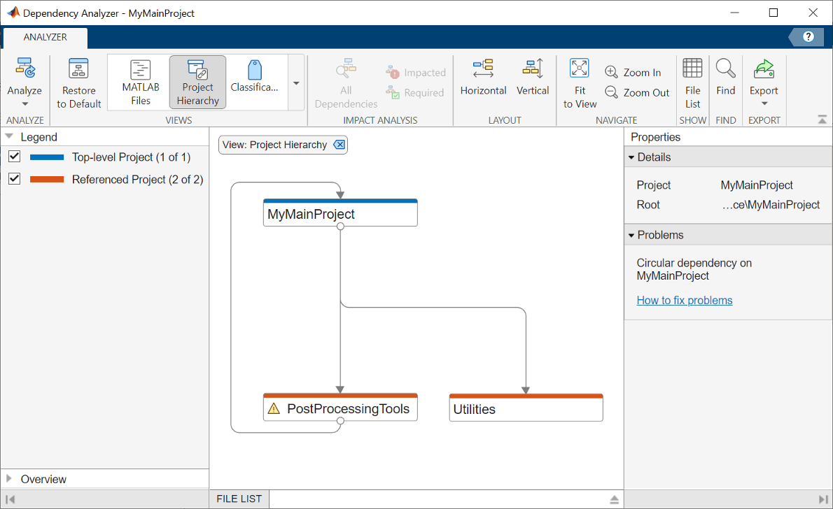
Project Hierarchy view shows the relations between the different projects in the hierarchy. Warning about the circular dependency in the Properties panel on the right.

Unit Testing Framework: Run tests interactively by using Test Browser

The Test Browser app enables you to run script-based, function-based, and class-based tests interactively. You can use the test browser to:

  • Create a test suite from files and folders.

  • Run all or part of the specified tests.

  • Access diagnostics and debug test failures.

  • Customize a test run with options, such as running tests in parallel (requires Parallel Computing Toolbox) or specifying a level of test output detail.

  • Generate an HTML code coverage report for MATLAB source code.

For more information, see Run Tests Using Test Browser.

Unit Testing Framework: Programmatically access code coverage results

You can use the matlab.unittest.plugins.codecoverage.CoverageResult class to programmatically access the results of code coverage analysis for your source code. To generate and access the coverage results, create a CodeCoveragePlugin instance using a CoverageResult object, and add the plugin to the test runner. After the test run, the Result property of the CoverageResult object holds the coverage results as an array of matlab.coverage.Result objects. Each element of the array provides information about one of the files in your source code that was covered by the tests.

For more information, see Collect Statement and Function Coverage Metrics for MATLAB Source Code.

Unit Testing Framework: Temporarily set environment variables

The matlab.unittest.fixtures.EnvironmentVariableFixture class provides a fixture for setting an operating system environment variable. Once the testing framework tears down the fixture, the fixture restores the environment variable to its original state.

Unit Testing Framework: Test for handle validity

The matlab.unittest.constraints.IsValid class provides a constraint to test if a handle array is valid. The constraint is satisfied if all array elements are valid handles.

Unit Testing Framework: Write text to files in thread-based environment

You can use the ToFile and ToUniqueFile classes in a thread-based environment to write text to UTF-8 encoded files.

Unit Testing Framework: Use renamed classes in testing and other automated workflows

To reflect support for additional automated workflows, a group of matlab.unittest classes have been renamed. For example, matlab.unittest.Verbosity is now named matlab.automation.Verbosity.

This table shows the affected classes and their new names. The behavior of these classes remains the same, and existing instances of these classes in your code continue to work as expected. There are no plans to remove support for existing instances of these classes.

R2022b and EarlierStarting in R2023a
matlab.unittest.Verbositymatlab.automation.Verbosity
matlab.unittest.diagnostics.Diagnosticmatlab.automation.diagnostics.Diagnostic
matlab.unittest.diagnostics.DiagnosticResultmatlab.automation.diagnostics.DiagnosticResult
matlab.unittest.diagnostics.DisplayDiagnosticmatlab.automation.diagnostics.DisplayDiagnostic
matlab.unittest.diagnostics.FileArtifactmatlab.automation.diagnostics.FileArtifact
matlab.unittest.diagnostics.FunctionHandleDiagnosticmatlab.automation.diagnostics.FunctionHandleDiagnostic
matlab.unittest.diagnostics.StringDiagnosticmatlab.automation.diagnostics.StringDiagnostic
matlab.unittest.plugins.OutputStreammatlab.automation.streams.OutputStream
matlab.unittest.plugins.ToFilematlab.automation.streams.ToFile
matlab.unittest.plugins.ToStandardOutputmatlab.automation.streams.ToStandardOutput
matlab.unittest.plugins.ToUniqueFilematlab.automation.streams.ToUniqueFile

App Testing Framework: Test context menus within labels

You can use the chooseContextMenu method to test a right-click that opens a context menu within label components. For example, assign a context menu with two items to a label, and then choose the first menu item.

fig = uifigure;
lbl = uilabel(fig);

cm = uicontextmenu(fig);
m1 = uimenu(cm,Text="Menu1");
m2 = uimenu(cm,Text="Menu2");
lbl.ContextMenu = cm;

testCase = matlab.uitest.TestCase.forInteractiveUse;
testCase.chooseContextMenu(lbl,m1)

 Performance Testing Framework: Use fewer samples to meet the objective margin of error

The default number of times that the framework exercises the test code to warm it up in a frequentist time experiment (created using either the runperf function or the limitingSamplingError static method) has increased from four to five. This change results in typically fewer samples required to meet the objective relative margin of error.

 Compatibility Considerations

If your code relies on the previous default value, you might need to update your code. For example, if you use warmupTable = results(1).TestActivity(1:4,:) to create a table of warm-up measurements, replace 4 with 5. Also, if you want to keep using the previous default value, explicitly specify the value in your code. This table shows an example of how to update code that runs tests using four warm-up measurements.

BeforeAfter
import matlab.perftest.TimeExperiment
experiment = TimeExperiment.limitingSamplingError;
results = run(experiment,mySuite);
import matlab.perftest.TimeExperiment
experiment = TimeExperiment.limitingSamplingError("NumWarmups",4);
results = run(experiment,mySuite);

 Functionality being removed or changed

TaskAction constructor method has been removed

Errors

The constructor method of the matlab.buildtool.TaskAction class has been removed. To specify a task action, use a function handle instead of the constructor method. This table shows an example of how to update code that calls the TaskAction constructor method.

BeforeAfter
import matlab.buildtool.Task
import matlab.buildtool.TaskAction

plan = buildplan;
plan("test") = Task( ...
    Actions=TaskAction( ...
    @(~)assertSuccess(runtests(IncludeSubfolders=true)),Name="Testing"));
import matlab.buildtool.Task

plan = buildplan;
plan("test") = Task( ...
    Actions=@(~)assertSuccess(runtests(IncludeSubfolders=true)));

External Language Interfaces

Publish C++ Interface: Publish interface for C++ library in Live Editor

The clibPublishInterfaceWorkflow function creates a live script that guides you through the steps to publish a MATLAB interface to a C++ library. For more information, see Steps to Publish a MATLAB Interface to a C++ Library and Generate C++ Interface.

Interface to C++ Library: Execute C++ library functions out-of-process

Run C++ library functions in processes that are separate from the MATLAB process. For more information, see Load C++ Library In-Process or Out-of-Process. Use out-of-process mode to call functions in third-party libraries that are not compatible with MATLAB. Publishers can use this mode while developing an interface, eliminating the need to restart MATLAB while testing.

Interface to C++ Library: Support for default arguments

If a C++ function is defined with default arguments, then you can call the function without providing one or more trailing arguments. MATLAB supports default arguments for scalar integer and floating-point types.

The MATLAB interface to C++ libraries displays default arguments in function signatures in the library definition file and in the help text. For example, the argument arg for the function funcname has a default value of 5.

% C++ Signature: void funcname(double arg = 5.000000)

These calls to funcname produce the same result:

clib.libname.funcname
clib.libname.funcname(5)

For more information, see Call Function with Default Arguments.

Interface to C++ Library: Support for comments in function templates

The generated help text in a MATLAB interface to a C++ library includes Doxygen comments from template functions and template methods of a class. For information about viewing these comments, see Display Help for MATLAB Interface to C++ Library. For information about modifying comments when publishing an interface, see Publish Help Text for MATLAB Interface to C++ Library.

Publish C++ Interface: Put libraries on run-time path

Use the copyRuntimeDependencies function to copy dependent libraries to the run-time path so that they are available when you test. This function collects the necessary files for distributing to end users so that they do not have to set environment variables to call functions in the library. For information, see Set Up and Copy Run-Time Libraries.

Publish C++ Interface: Resolve multiple redefinition and unresolved external symbol errors

Error messages for multiple redefinition and unresolved external symbol compiler errors provide additional help for you to resolve the error. For more information, see Resolve Build Error: Multiple Redefinition Linker Errors and Resolve Build Error: Unresolved External Symbols.

Publish C++ Interface: Information to debug C++ library functions

You can debug C++ library functions by using a debug-version of the MATLAB interface to the library. For steps to build a debug-version, see Debug C++ Library from MATLAB Interface.

Publish C++ Interface: Support for MATLAB operators for C++ methods

In a MATLAB interface to a C++ library, MATLAB operators are supported when corresponding methods are defined in a C++ class.

Operation in MATLAB

Method to Define in C++ Class

a < blt(a,b)
a > bgt(a,b)
a <= ble(a,b)
a >= bge(a,b)
a ~= bne(a,b)
a == beq(a,b)

Java Interface: Support for Java 11 JDK and JRE

MATLAB supports Java 11 JDK™ and JRE. To use this version, located in the folder jre_path, call the jenv function. At the MATLAB prompt, type:

e = jenv("jre_path")

You might have to restart your MATLAB session to change to this version.

Java Interface: jenv and matlab_jenv provide environment information

The jenv function returns a JavaEnvironment object, which contains information about the Java program on your system. The matlab_jenv command displays Java environment information at the operating system prompt, but it does not return the information.

Python Interface: Convert between MATLAB datetime and Python datetime, NumPy datetime64 types

You can convert between MATLAB datetime values and Python datetime or NumPy datetime64 values. For examples, see Use MATLAB datetime Types with Python.

Python Interface: Convert between MATLAB duration and Python timedelta, NumPy timedelta64 types

You can convert between MATLAB duration values and Python timedelta or NumPy timedelta64 values. For examples, see Use MATLAB duration Types with Python.

Python Objects: Use Python objects as keys in dictionary

You can use Python objects as keys in dictionaries. For more information about dictionary keys, see dictionary.

.NET Interface: Convert between MATLAB dictionary and .NET System.Collections.Generic.Dictionary objects

You can convert a MATLAB dictionary to a .NET dictionary. For more information, see Pass Data to .NET Objects.

To explicitly create a .NET dictionary from a MATLAB dictionary, call the NET.createDictionary function.

To convert a .NET dictionary to a MATLAB dictionary, see How MATLAB Handles .NET Dictionary Objects.

.NET Objects: Use .NET objects as keys in dictionary

You can use .NET objects as keys or values in dictionaries. For more information about dictionary keys, see dictionary.

.NET Engine: Support for MATLAB structs

Use the .NET MathWorks.MATLAB.Types.MATLABStruct class to represent MATLAB struct objects. For examples, see Use MATLAB Structures in .NET.

 Perl 5.36.0: MATLAB support on Windows

As of R2023a, MATLAB on Windows ships with an updated version of Perl, version 5.36.0, and supports an updated version of HTML::Parser, version 3.78.

 Compatibility Considerations

If you use the perl command on Windows platforms, see https://www.perl.org/ for information about using this version of the Perl programming language. For a standard distribution of HTML::Parser, source code, and information about using HTML::Parser, see https://metacpan.org/pod/HTML::Parser.

 Compiler support changed for building C and C++ interfaces, MEX files, and standalone MATLAB engine and MAT-file applications

SupportCompilerPlatform

Added

Intel oneAPI 2023 with Microsoft Visual Studio 2019 and 2022 for C, C++, and Fortran

Windows
macOS

Added

Intel oneAPI 2022 with Microsoft Visual Studio 2017, 2019, and 2022 for C, C++, and Fortran

Windows

Added

MinGW-w64 version 8.1 compiler. For installation instructions, see this MATLAB Answers™ article FAQ: How do I install the MinGW compiler?

Windows

To be phased out

Intel Parallel Studio XE for C/C++

Windows

For continued support for building your applications, consider upgrading to a supported compiler. For an up-to-date list of supported compilers, see Supported and Compatible Compilers.

 Functionality being removed or changed

Python version 2.7 is no longer supported

Errors

Support for Python version 2.7 is discontinued. For continued support for your applications, upgrade to a supported version of Python. For supported version information, see Versions of Python Compatible with MATLAB Products by Release.

-std=c++11 flag is no longer included in MEX options files

Behavior change

MEX options files for building C++ code with MinGW and Linux compilers no longer include the CXXFLAGS option -std=c++11.

MEX options files for macOS compilers include the CXXFLAGS option -std=c++14 instead.

However, you can still build MEX files with the -std=c++11 option. For example, build the MEX file myFunc.cpp with that option.

mex myFunc.cpp 'CXXFLAGS=$CXXFLAGS -std=c++11'

Continuous console and writer output for MATLAB API for Java functions

Behavior change

When you call a MATLAB function that displays output using one of the evaluate functions in com.mathworks.engine.MatlabEngine, then the output continuously displays on the console and writer output stream. This behavior applies to feval, fevalAsync, eval, and evalAsync.

Before R2023a, the output displays after the MATLAB function completes.

.NET Interface: Dictionary with cell types map to .NET System.Object instead of System.Object[]

Behavior change

A MATLAB dictionary with entries of type cell are converted to a .NET dictionary with entries of type System.Object. Previously, the conversion was to System.Object[]. For more information, see Pass Data to .NET Objects and How MATLAB Handles .NET Dictionary Objects.

Hardware Support

Support for MJPEG format in USB Webcams on Windows

Starting R2023a, the MATLAB Support Package for USB Webcams installed on a Windows machine supports the MJPEG image format. The MJPEG format provides improved frame rates for acquiring high-resolution images from a USB webcam.

Support for 32-bit Debian Bullseye on Raspberry Pi

Raspberry Pi Blockset now supports 32-bit Debian Bullseye for MATLAB desktop and MATLAB Online. You can now customize Debian Bullseye running on your Raspberry Pi hardware to make it compatible with MATLAB while doing the Hardware Setup.

Support for Raspberry Pi Zero 2 W and Raspberry Pi Compute Module 4

You can now use the Raspberry Pi Blockset with Raspberry Pi Zero 2 W and Raspberry Pi Compute Module 4 for MATLAB desktop and MATLAB Online.

R2022b

New Features, Bug Fixes, Compatibility Considerations

Environment

Live Editor Controls: Add numeric spinners to increment and decrement variable values in live scripts

You can add numeric spinners to your live scripts to interactively increment and decrement the value of variables. To add a numeric spinner, go to the Live Editor tab, and in the Code section, click Control. Then, select Numeric Spinner.
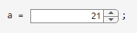
Numeric spinner with a value of 21, assigned to the variable a

For more information, see Add Interactive Controls to a Live Script.

Live Editor Tasks: Specify what code to run when control value changes

By default, when you change a parameter in a Live Editor task, the Live Editor runs the section that contains the task. You can now configure a Live Editor task to run all sections, run the current section and all modified sections above that section, run the current section and all remaining sections, or to do nothing.

To configure the task, click the Options button () in the top-right corner of the task. Select Autorun and then select from the available options. For more information, see Add Interactive Tasks to a Live Script.

Suggestions and Completions: Change when to show suggestions and how to accept them

Starting in R2022b, you can use Ctrl+Space to show code suggestions in the Editor, Live Editor, App Designer, and MATLAB Online Command Window. In addition, you can change when to show suggestions and how to accept them. On the Home tab, in the Environment section, click Preferences. Select Editor/Debugger > Automatic Completions and in the Suggestions and completions section, adjust one or more of the options:

  • To disable showing suggestions automatically, clear the Show suggestions automatically option.

  • To disable showing suggestions after you press the Tab key, clear the Use tab to show suggestions (in addition to ctrl+space) option. When this option is cleared, you can still show suggestions by typing Ctrl+Space.

  • To disable accepting a suggestion using the Right Arrow key, clear the Use right arrow to accept suggestions (in addition to tab and enter) option. When this option is cleared, you can still accept a suggestion using the Tab and Enter keys.

For more information, see Code Suggestions and Completions.

Search in MATLAB Online: Access toolstrip actions, preferences, and Help Center resources using search

In MATLAB Online, you can now use the Search box in the top-right corner of the desktop to easily access toolstrip actions, preferences, and Help Center resources such as functions, blocks, examples, and answers. To navigate to the Search box using a keyboard, press Ctrl+Shift+Space (or Command+Shift+Space on macOS systems).

For example, to restore the MATLAB desktop to its default layout, enter the word layout in the Search box. In the list of results, select the Layout - Two Column (Default) toolstrip action.
Search box containing the word layout and a list of search results including toolstrip actions, functions, blocks, and examples

System Theme in MATLAB Online: Change colors of MATLAB desktop to match operating system color scheme

Windows and macOS systems support light and dark color schemes. Starting in R2022b, MATLAB Online is configured to match the current operating system color scheme by default using the system theme. If the selected color scheme for the operating system changes, the colors of the MATLAB desktop change to match the new scheme.

To change the selected theme, on the Home tab, in the Environment section, click Preferences. Select MATLAB > Appearance and select a theme from the Theme field. For more information, see Change Desktop Colors.

If you customize the colors of the MATLAB desktop and then the MATLAB desktop theme changes to a new theme or to match a change to the operating system color scheme, your customizations will be lost. To avoid unexpectedly losing color customizations when the operating system color scheme changes, select the Light or Dark option from the Theme field before making any color customizations.

Help Center: View documentation for all products and determine which products are installed

When viewing the documentation from an installed version of MATLAB, you can now view the documentation for all products. Previously, you could view only the documentation for installed products. The Help browser indicates installed products using a green bar to the left of the product name or its category.
Help browser showing the documentation by category. The MATLAB; AI, Deep Learning, Statistics and Data Science; and Mathematics and Optimization categories have a green bar to the left of their names.

To view the list of installed products, select Product List at the top left of the Help browser. The Help browser displays the list of products that are installed for the current version of MATLAB. If MATLAB is configured to display the web documentation (default), the Help browser also displays the list of products that are not installed.
Help browser showing the Contents panel on the left with the Product List selected. The Product List includes the list of products that are installed, followed by the list of products that are not installed.

unsetenv Function: Remove environment variable

You can remove an environment variable from the operating system by using the unsetenv function.

isenv Function: Determine if environment variable exists

To determine if an environment variable exists in the operating system, you can use the isenv function.

Comparison Tool: Compare MAT files, FIG files, live scripts, and live functions in MATLAB Online

Starting in R2022b, you can compare MAT and FIG files in MATLAB Online. You also can compare live scripts and functions.

You can access the comparison tool from:

  • The MATLAB Current Folder browser context menu

  • The Current Project browser context menu

  • The MATLAB Command Window by using the visdiff function

 Functionality being removed or changed

matlab.keyboard.ShowAutomatically and matlab.commandwindow.ShowCompletionsAutomatically settings have been removed

Errors

The matlab.keyboard.ShowAutomatically and matlab.commandwindow.ShowCompletionsAutomatically settings have been removed. Use the matlab.editor.suggestions.ShowAutomatically and matlab.commandwindow.suggestions.ShowAutomatically settings instead.

To update your code, change instances of the setting matlab.keyboard.ShowAutomatically to matlab.editor.suggestions.ShowAutomatically and instances of the setting matlab.commandwindow.ShowCompletionsAutomatically to matlab.commandwindow.suggestions.ShowAutomatically. For more information, see matlab.editor and matlab.commandwindow.

lookfor function no longer searches third-party and user-authored help text

Behavior change

The lookfor function no longer searches help text in third-party and user-authored MATLAB program files. In previous releases, lookfor searches all MATLAB program files on the path, including third-party and user-authored program files.

To search the documentation including third-party and custom documentation, use the docsearch function instead. Alternatively, you can use the find features in the Current Folder browser. For example, you can look for all occurrences of a specified word in all the MATLAB program files in the current folder and its subfolders. For more information, see Find Files and Folders.

Language and Programming

dictionary Object: Map unique keys to values for fast lookup

Dictionaries are useful for fast lookup of values in a large data set. A dictionary stores data as values, which can be accessed using corresponding unique keys. For example, create a dictionary that contains three key-value pairs.

d = 

  dictionary (string ⟼ double) with 3 entries:

    "Unicycle" ⟼ 1
    "Bicycle"  ⟼ 2
    "Tricycle"  ⟼ 3

Use a key to look up the corresponding value in a dictionary.

d("Bicycle")
ans =

     2

In almost all use cases, dictionary performs faster than containers.Map. For more information, see dictionary.

Output Argument Validation: Validate output arguments in functions and class methods

You can now define output argument blocks for functions and class methods. Use many of the available argument validation techniques on output arguments, including size and data type restrictions as well as validation functions. Input validation checks that function users provide valid inputs. Output validation helps function authors ensure that their functions return the expected types of outputs. It also helps identify errors in the function definition that cause unexpected outputs.

For example, realPolyRoots is based on the roots function. The input argument block restricts the degree of the input polynomial to a quadratic. The output arguments block only allows the function to return results when the roots are real valued.

function r = realPolyRoots(p)
    arguments (Input)
        p (1,3)
    end
    
    arguments (Output)
        r {mustBeReal}
    end
 
    r = roots(p);
end

Calling realPolyRoots on x2 – 1 (p = [1 0 -1]) returns roots 1 and –1, but calling the function on x2 + 1 errors.

realPolyRoots([1 0 1])
Invalid output 'r'. Value must be real.
 
Error in realPolyRoots (line 11)
end 

For more information, see Function Argument Validation.

Code Analyzer App: Identify code issues

The MATLAB Code Analyzer is now available as an app. Use the Code Analyzer app to identify issues in code and implement suggested fixes when possible.

codeIssues Object: Identify and store code issues from one or more files

Create a codeIssues object to identify and store code issues found within specified files. When displayed in the Command Window, the codeIssues object shows the location of identified issues in the code.

Custom Compact Display: Live Editor, Variables editor, and Workspace browser follow CustomCompactDisplayProvider implementations

Starting in R2022b, the Live Editor, the Variables editor in MATLAB Online, and the single-line Value field in the Workspace browser in MATLAB Online follow rules for customized object display implemented using the matlab.mixin.CustomCompactDisplayProvider class. For more information on custom compact displays, see Custom Compact Display Interface.

Customized Dot Indexing: New methods handle parentheses-dot combinations

The matlab.mixin.indexing.RedefinesDot class has two new concrete methods—parenDotAssign and parenDotListLength—that handle built-in parentheses indexing immediately followed by customized dot indexing, such as obj(idx).prop = val. The two methods have default implementations that provide the expected behavior, but you can override them if needed.

 Functionality being removed or changed

isequal and isequaln return false when comparing empty arrays of the same size but of different classes

Behavior change

Previously, isequal and isequaln returned true when comparing two or more empty object arrays of the same size, regardless of the class of the objects. Starting in R2022b, both functions return false when comparing empty object arrays of the same size but different classes.

Defining classes and packages: Using schema.m will not be supported in a future release

Still runs

Support for classes and packages defined using schema.m files will be removed in a future release. Replace existing schema-based classes with classes defined using the classdef keyword.

Multiple repeating arguments blocks throw an error on empty blocks

Behavior change

If a function contains multiple arguments blocks with the Repeating property, MATLAB now throws an error regardless of if the blocks are empty or have declared repeating arguments. Previously, MATLAB threw an error only if there was more than one repeating block with repeating arguments specified.

Multiple repeating arguments validate individual elements of all repeating arrays together

Behavior change

If a function contains multiple arguments with the Repeating property, argument validation functions that accept multiple inputs will now make element-wise comparisons. For example, this function uses a validation function with multiple repeating arguments as inputs.

function MyFoo(x,y)
    arguments(Repeating)
       x
       y {mustBeGreaterThan(x,y)}
    end
end

The validation function mustBeGreaterThan(x,y), validates each single element of y against a single corresponding element of x. Previously, mustBeGreaterThan(x,y) validated a single element of y against the entire cell array of repeating values of x.

Dynamic Regular Expressions: Commands in replacement expressions now check only the local workspace for variables

Behavior change

Commands in replacement expressions using the syntax ${cmd} will only check the local workspace for variables. Caller and global workspaces will not be available to commands in replacement expressions. This means that commands in replacement expressions now work in parfor loops.

Data Analysis

Data Cleaner App: Clean data in table

The Data Cleaner app supports importing and cleaning data in a table. You can access a table in the MATLAB workspace or import a table from a file. Previously, the app cleaned only timetable data.

You can open the Data Cleaner app from the MATLAB section of the apps gallery in the Apps tab. Alternatively, enter dataCleaner in the MATLAB Command Window.

Data Cleaner App: View sparklines and summary statistics

The Data view in the Data Cleaner app displays sparklines and summary statistics to quickly visualize and interpret the data in each table or timetable variable. Show more information related to specific points by pointing to a sparkline.
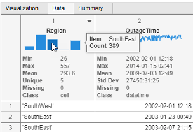
Data view in the Data Cleaner app showing a sparkline and summary statistics for timetable variables. A tooltip for the Region variable sparkline indicates that there are 389 outages in the SouthEast region.

stackedplot Function: Plot data from multiple tables or timetables

The stackedplot function can now plot variables from multiple input tables or timetables. In previous releases, stackedplot can plot variables only from a single table or timetable.

For example, to plot data from the two sample timetables indoors and outdoors, load the two MAT-files and then call stackedplot.

load indoors.mat
load outdoors.mat
stackedplot(indoors,outdoors)

If you specify multiple inputs, then they must be either all tables or all timetables.

To work with multiple inputs, stackedplot has new name-value arguments:

  • CombineMatchingNames — If true, then plot variables from different inputs but with the same names in the same y-axis. If false, then plot them in different y-axes.

  • LegendLabels — If specified, then create a legend with the specified labels instead of the names of the input tables or timetables.

  • LegendVisible — If "on", then display the legend. If "off", then hide the legend.

  • LegendOrientation — If "horizontal", then display the legend horizontally. If "vertical", then display the legend vertically.

detrend Function: Detrend tabular data

The detrend function can detrend data in a table or timetable.

When detrending table or timetable data, you can:

  • Specify tabular variables to detrend by using the DataVariables name-value argument.

  • Append or replace tabular variables with variables containing detrended data by using the ReplaceValues name-value argument.

  • Specify the sample points as a table variable by using the SamplePoints name-value argument. SamplePoints is not supported when the input data is a timetable.

rmoutliers Function: Define outlier locations, and optionally return outlier indicator, thresholds, and center value

When using the rmoutliers function, you can define the location of outliers in the input data with a known outlier indicator. Define outlier locations, rather than using an outlier detection method, by setting the OutlierLocations name-value argument to a logical array the same size as the input data.

Regardless of whether the outliers are defined or detected, the rmoutliers function can return a logical outlier indicator array indicating the locations of outliers in the input data.

rmoutliers can also return the lower threshold value, upper threshold value, and center value used by the outlier detection method. The code generated by the Clean Outlier Data task in the Live Editor includes the new output arguments.

mape and rmse Functions: Calculate error between forecast and actual data

Calculate the mean absolute percentage error and the root-mean-square error between arrays by using the mape and rmse functions, respectively. You can specify the dimensions to operate along, whether to include or omit zero values (mape only) or NaN values from the calculation, or a weighting scheme.

isuniform Function: Determine if vector is uniformly spaced

Determine if a numeric vector is uniformly spaced up to round-off tolerance by using the isuniform function. You can optionally return the step size between consecutive elements.

 Serial date numbers and date strings are not recommended

To represent dates and times in MATLAB, use the datetime, duration, and calendarDuration data types. The datetime data type represents points in time, and the duration and calendarDuration data types represent lengths of time. In particular, the datetime data type provides flexible date and time formats, storage out to nanosecond precision, and properties to account for time zones and daylight saving time.

 Compatibility Considerations

Serial date numbers and date strings are not recommended. As a consequence, MATLAB functions that create or modify serial date numbers or date strings, such the datenum and datestr functions, are not recommended.

MATLAB functions that accept serial date numbers or date strings as inputs also accept datetime arrays as inputs.

There are no plans to remove support for serial date numbers or date strings.

datetime and convertTo Functions: Convert between CDF TT2000 times and datetime arrays

The NASA Common Data Format (CDF) defines the CDF_TIME_TT2000 (or TT2000 for short) data type as a high-resolution time type that handles leap seconds for data in CDF files. TT2000 times represent the number of nanoseconds that have elapsed since J2000.

You can convert int64 arrays that represent TT2000 times to datetime arrays. To convert TT2000 times, call the datetime function with ConvertFrom set to "tt2000" and TimeZone set to "UTCLeapSeconds". To account for leap seconds, you must specify the time zone of the output datetime array.

X = int64([702077514184000000; ...
           702163914184000000; ...
           702250314184000000])
D = datetime(X,"ConvertFrom","tt2000","TimeZone","UTCLeapSeconds")

Also, you can convert datetime arrays to int64 arrays that represent TT2000 times. To convert datetime arrays, call the convertTo function using the "tt2000" option. To account for leap seconds, the input datetime array must have its time zone set to "UTCLeapSeconds".

D = datetime(2022,4,1:3,9,30,45, ...
             "TimeZone","UTCLeapSeconds")
X = convertTo(D,"tt2000")

Data Preprocessing Live Editor Tasks: Plot multiple table variables

These Live Editor tasks can plot multiple table variables:

For table or timetable data, to visualize all selected table variables at once in a tiled chart layout, set the Variable to display field.

Data Preprocessing Live Editor Tasks: Append cleaned table variables and specify logical tabular output

These Live Editor tasks can append cleaned table variables to the input table variables:

Additionally, in these Live Editor tasks, you can specify to output a table with logical variables:

To append cleaned table variables or specify a tabular output with logical variables, set the Output format field.

Clean Missing Data Live Editor Task: Plot nonnumeric table data, specify minimum number of missing entries, and use custom fill method

The Clean Missing Data task in the Live Editor can now plot nonnumeric data. To display a categorical histogram, select a nonnumeric input array or set the Variable to display field to a nonnumeric table variable containing categorical, string, cellstr, calendarDuration, or char data types.

You can specify a minimum number of missing entries required to remove a row of data. First, select the Remove missing cleaning method, and then specify the minimum number of missing entries by using the Min missing for removal field.

You can also specify a custom fill method for filling missing data. Select the Fill missing cleaning method, and then specify a custom fill method by selecting the Custom function cleaning method parameter and the local function or function handle option.

Clean Outlier Data Live Editor Task: Convert outliers to missing

Use the Clean Outlier Data task in the Live Editor to convert outlier data to missing data indicated by the value NaN. Convert outlier data to missing data by setting the Cleaning method field to Fill outliers and selecting the Convert to missing option.

Live Editor and Variables Editor: Control placement of missing values when sorting numeric data in MATLAB Online

In the Live Editor output and Variables editor in MATLAB Online, you can control the placement of missing values (NaN, NaT, <undefined>, and missing) when sorting rows of numeric data.

For example, to place missing elements first, on the Home tab, in the Environment section, click Preferences. Select MATLAB > Variables and set Placement of missing values to first.

In the Variables editor, you can also control missing value placement using the Variable tab. In the Transform section, from the Sort list, select an option for Missing Placement.

Variables Editor: View sparklines and summary statistics for tabular data in MATLAB Online

The Variables editor in MATLAB Online now displays sparklines and summary statistics to quickly visualize and interpret the data in each table or timetable variable. Show more information related to specific points by pointing to a sparkline. Show or hide the sparklines or summary statistics using the Display section in the View tab.
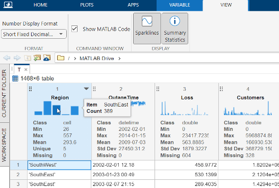
Variables editor view of a timetable of power outage data with a sparkline and summary statistics for each table variable. A tooltip for the Region variable sparkline indicates that there are 389 outages in the SouthEast region.

Variables Editor: Navigate variable with Find and Go To dialog boxes in MATLAB Online

In the Variables editor in MATLAB Online, search for any text in the current variable or selection. On the Variable tab, in the Navigate section, click Find. You can also use the Ctrl+F keyboard shortcut. In the Find dialog box, enter the text that you want to search for and use the arrow buttons to search backward or forward through the current variable. You can also change how the Variables editor searches for text by selecting the match case, whole word, or regular expression search options.

Additionally, in the Variables editor in MATLAB Online, navigate to a particular location in the current variable. On the Variable tab, in the Navigate section, click Go To. You can also use the Ctrl+G keyboard shortcut. In the Go To dialog box, specify with numeric or text indices the row and column that you want to navigate to.

Variables Editor: Interactively save logical indices of data selection in MATLAB Online

In the Variables editor in MATLAB Online, create a new logical variable indicating the indices of the selected data by right-clicking the selection or by clicking New from Selection in the Variable tab.

For tabular data:

  • Append a logical table variable indicating the selection

  • Create a logical column vector in the workspace indicating the selected rows

  • Create a logical row vector in the workspace indicating the selected columns

For all other data types except for structure arrays and objects:

  • Create a logical matrix in the workspace indicating the selection

  • Create a logical column vector in the workspace indicating the selected rows

  • Create a logical row vector in the workspace indicating the selected columns

Variables Editor: Replace tabular data with empty arrays in MATLAB Online

In the Variables editor in MATLAB Online, replace the current selection of table or timetable elements with empty 0-by-0 arrays by pressing the Delete key or by right-clicking the selection and selecting Replace with Empty. The class of an empty array is determined by the class of the table variable.

Previously, you could interactively replace the current data selection with empty arrays for nontabular data only.

 Functionality being removed or changed

Character arrays have no standard missing value

Behavior change

For these functions, character arrays have no default definition of a standard missing value:

Blank char elements (' ') are treated as nonmissing. For example, ismissing(['a'; ' ']) returns logical array [0; 0]. In previous releases, it returns [0; 1].

To treat blank character array elements as missing, use an indicator. For example, ismissing(['a'; ' '],' ') specifies a blank char as a missing value and returns [0; 1].

Join Tables Live Editor task automatically selects merging variables based on scoring algorithm

Behavior change

If the Join Tables Live Editor task fails to automatically select the first pair of merging variables based on row labels or variable names, then it tries to select them based on a scoring algorithm. The Join Tables task selects and tests candidate pairs of merging variables using these steps:

  1. Select row names (in a table) or row times (in a timetable) as the first pair of merging variables.

  2. If step 1 fails, then select variables with names that exactly match as the first pair.

  3. If steps 1 and 2 fail, then score pairs of variables using the scoring algorithm. Select the pair of variables with the highest score as the first pair of merging variables.

  4. If all previous steps fail, then select the first items in the Merging variable drop-down lists as the first pair of merging variables.

In previous releases, step 3 was to select the pair of variables whose names gave the best partial match as the first pair of merging variables.

Java objects open in an improved Property Inspector

Behavior change

Java objects now open in an improved Property Inspector that is consistent with the one used for graphics and other handle objects. For example, view and edit the properties of a Java object using the improved Property Inspector.

myDate = java.util.Date;
inspect(myDate)
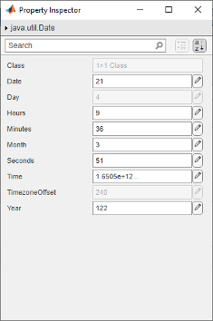
Improved Property Inspector for Java objects

Calling head and tail functions without specified output arguments does not store output in ans

Behavior change

When you call the head and tail functions without specified output arguments, they display the selected rows of input tables, but they do not store output in the ans variable. In previous releases, calling head and tail without specified output arguments causes output to be stored in ans.

Calling head and tail in a live script is usually not recommended. Instead, display the table or timetable by typing the variable name with no semicolon. The Live Editor provides a widget that enables you to examine the entire table or timetable. However, if you do call head or tail in a live script, you should assign the output to a variable so that the live script creates a widget for the output.

addtodate function is not recommended

Still runs

There are no plans to remove addtodate. However, the datetime, duration, and calendarDuration data types are recommended instead. The datetime data type provides flexible date and time formats, storage out to nanosecond precision, and properties to account for time zones and daylight saving time. You can add lengths of time to datetime values by using duration values (for hours, minutes, and seconds) or calendarDuration values (for calendar years, quarters, months, weeks, or days).

For example, convert a serial date number to a datetime value. Then add an array of hours, in 4-hour increments, by using the hours function to create an array of duration values. The result is an array of datetime values.

d = 738522;
d = datetime(d,"ConvertFrom","datenum")
d = datetime
   01-Jan-2022
d = d + hours(0:4:12)
d = 1x4 datetime array
   01-Jan-2022 00:00:00   01-Jan-2022 04:00:00   01-Jan-2022 08:00:00   01-Jan-2022 12:00:00

Add 3 calendar months and 2 calendar weeks to a datetime value that represents January 1, 2022, 12:00 p.m. by using the calmonths and calweeks functions to create calendarDuration values. The result is a datetime value that represents April 15, 2022, 12:00 p.m.

d = datetime("01-Jan-2022 12:00:00");
d = d + calmonths(3) + calweeks(2)
d = datetime
   15-Apr-2022 12:00:00

clock function is not recommended

Still runs

There are no plans to remove clock. However, the datetime function is recommended instead. The datetime data type provides flexible date and time formats, storage out to nanosecond precision, and properties to account for time zones and daylight saving time.

To return the current time as a datetime value, call datetime with "now" as the input argument.

d = datetime("now")
d = datetime
   15-Apr-2022 15:53:28

date function is not recommended

Still runs

There are no plans to remove date. However, the datetime function is recommended instead. The datetime data type provides flexible date and time formats, storage out to nanosecond precision, and properties to account for time zones and daylight saving time.

To return the current date as a datetime value, call datetime with "today" as the input argument.

d = datetime("today")
d = datetime
   15-Apr-2022

datenum function is not recommended

Still runs

There are no plans to remove datenum. However, the datetime, duration, and calendarDuration data types are recommended instead. The datetime data type provides flexible date and time formats, storage out to nanosecond precision, and properties to account for time zones and daylight saving time. MATLAB functions that accept serial date numbers as inputs also accept datetime arrays as inputs.

To convert a serial date number to a datetime value, call datetime with the ConvertFrom name-value argument set to "datenum".

d = 738522;
d = datetime(d,"ConvertFrom","datenum")
d = datetime
   01-Jan-2022

datestr function is not recommended

Still runs

There are no plans to remove datestr. However, the string and char functions are recommended instead for converting datetime arrays to text. The datetime data type provides flexible date and time formats, storage out to nanosecond precision, and properties to account for time zones and daylight saving time.

For example, represent the current date and time as a datetime value. Then convert it to a string.

d = datetime("now")
d = datetime
   15-Apr-2022 15:53:28
str = string(d)
str = 
    "15-Apr-2022 15:53:28"

Using datevec function on serial date numbers is not recommended

Still runs

Using datevec with serial date numbers as inputs is not recommended. Use the datetime data type to represent points in time instead. The datetime data type provides flexible date and time formats, storage out to nanosecond precision, and properties to account for time zones and daylight saving time.

To split datetime values into date and time components, use the hms, ymd, or datevec functions, or use the Year, Month, Day, Hour, Minute, and Second properties of datetime values.

For example, call datevec on a datetime value that represents the current date and time.

d = datetime("now")
d = datetime
   15-Apr-2022 15:53:28
format shortg
dateVector = datevec(d)
dateVector =

        2022           4          15          15          53          28

To access one component, use the corresponding datetime property. For example, get the value of the Month property of d.

monthValue = d.Month
monthValue =

     4

etime function is not recommended

Still runs

There are no plans to remove etime. However, the datetime, duration, and calendarDuration data types are recommended instead. The datetime data type provides flexible date and time formats, storage out to nanosecond precision, and properties to account for time zones and daylight saving time.

To calculate the elapsed time between two datetime values, either subtract one from the other or use the between function. For example, subtract the start of today from the current date and time. Return the elapsed time as a duration value.

startOfToday = datetime("today")
currentTime = datetime("now")
startOfToday = datetime
   15-Apr-2022

currentTime = datetime
   15-Apr-2022 15:53:28
elapsedTime = currentTime - startOfToday
elapsedTime = duration
   15:53:28

To return elapsed time as a calendarDuration value, use between.

d1 = datetime("2022-01-01")
d2 = datetime("now")
elapsedTime = between(d1,d2)
elapsedTime = calendarDuration
   6mo 18d 13h 19m 18.5561949999974s

now function is not recommended

Still runs

There are no plans to remove now. However, the datetime function is recommended instead. The datetime data type provides flexible date and time formats, storage out to nanosecond precision, and properties to account for time zones and daylight saving time.

To return the current date and time as a datetime value, call datetime. You can call it without any input arguments, or with "now" as the input argument.

d = datetime
% or
d = datetime("now")
d = datetime
   15-Apr-2022 15:53:28

Data Import and Export

Parquet: Use Parquet files containing nested structured data

Write nested table and timetable variables to Parquet files using parquetwrite. Read nested data from Parquet files as nested tables using parquetread and parquetDatastore.

SequentialDatastore Object: Sequentially read data from multiple datastores

Sequentially read data from multiple underlying datastores without concatenation using a SequentialDatastore object. Create a SequentialDatastore object using the combine function with the ReadOrder name-value argument.

Datastores: Create subsets of arbitrarily nested transformations and combinations of datastores

Create subsets of data from TransformedDatastore, CombinedDatastore, and SequentialDatastore objects using the subset function. You can subset these datastore objects only if their underlying datastores are subsettable (able to be subset). The underlying datastores can also be transformations or combinations of datastores that are subsettable.

Test whether you can create subsets of these datastore objects using the isSubsettable function. isSubsettable returns true when the underlying datastore can be subset.

Parallel Processing: Use low-level file I/O operations in thread-based environments

Use low-level file operations, such as fread, in thread-based environments. Parallel processing results in improved performance when reading data, especially with remote data. For a list of low-level functions that support thread-based environments, see Low-level File I/O.

CDF Interface: Read CDF_INT8 and CDF_TIME_TT2000 data

You can now use cdfinfo, cdfread, and the low-level CDF package functions to display and read CDF_INT8 and CDF_TIME_TT2000 variables and attributes from CDF datasets.

  • High-level interface — cdfread reads CDF_TIME_TT2000 data as datetime values by default. To read the data as int64 values, use the new name-value argument DatetimeType.

  • Low-level interface — CDF_TIME_TT2000 data is read as int64 values.

Use these two new functions to convert to and from CDF_TIME_TT2000 int64 timestamps:

  • cdflib.computeTT2000 — Calculate a CDF_TIME_TT2000 int64 timestamp from an input vector of UTC-based date and time components.

  • cdflib.breakdownTT2000 — Decompose a CDF_TIME_TT2000 int64 timestamp into an output vector of UTC-based date and time components.

imwrite Function: Use datetime values to write metadata for PNG images

You can write PNG image metadata using datetime values by specifying the CreationTime and ImageModTime name-value arguments with the imwrite function.

Image File Format Libraries: LibTIFF library upgraded to version 4.4.0

The LibTIFF library is upgraded to version 4.4.0.

Scientific File Format Libraries: HDF4 and HDF-EOS2 libraries are upgraded

The HDF4 library is upgraded to version 4.2.15, and the HDF-EOS2 library is upgraded to version 3.0.

 Functionality being removed or changed

NetCDF Interface: Use Fletcher32 checksum filter only with fixed-length data types

Behavior change

The Fletcher32 checksum filter can be used only with fixed-length data types and generates an error if you apply it to variables of type NC_STRING or NC_VLEN. Previously, if you applied the Fletcher32 filter to datasets that included NC_STRING or NC_VLEN data, the filter was silently ignored.

Use system web browser when opening links to external sites (recommended) preference has been removed

Behavior change

The Use system web browser when opening links to external sites (recommended) preference has been removed. Open all external sites using your system web browser.

Previously, you could use this preference to specify whether to open external sites using the system web browser or the MATLAB web browser.

Mathematics

pagenorm Function: Calculate norms using pages of N-D arrays

Use the pagenorm function to calculate vector and matrix norms of the pages of N-D arrays. In this context, the N-D array is treated as a container for several 2-D matrices. This function is particularly useful for calculating error metrics for the outputs of other page-wise functions, such as pagesvd and pagemldivide.

 Functionality being removed or changed

"0" syntaxes of qr, gsvd, and svd are not recommended for economy-size decompositions

Still runs

These qr, gsvd, and svd syntaxes for performing economy-size decompositions are no longer recommended:

  • [___] = qr(A,0) and [___] = qr(S,B,0)

  • [U,V,X,C,S] = gsvd(A,B,0)

  • [___] = svd(A,0)

There are no plans to remove support for the "0" syntax. However, using the "econ" option to perform economy-size decompositions with these functions is recommended instead.

gsvd output sizes are based on numerical rank of [A; B]

Behavior change

With the function call [U,V,X,C,S] = gsvd(A,B), where A is m-by-p and B is n-by-p, the gsvd function returns:

  • X as p-by-q

  • C as m-by-q

  • S as n-by-q

Additionally, with one output argument, the function call sigma = gsvd(A,B) returns a vector of the generalized singular values with length q.

The behavior change is that in all of these cases q is now equal to the numerical rank of [A; B]. The numerical rank is calculated from the QR factorization of [A; B]. This change ensures that nonzero elements of C and S are uniquely determined.

Previously, the value of q was min(m+n,p), and gsvd returned extra columns (or elements) in the outputs when [A; B] was not full rank.

Graphics

Plotting Table Data: Create stem, stairstep, and geographic plots by passing tables directly to plotting functions

Create plots by passing a table directly to any of these functions: stem, stem3, stairs, geoplot, and geoscatter. If you create any of these plots with a table and then add a legend, the legend items are automatically labeled with the table variable names. If you create a stem or stairstep plot, the axis labels are automatically set to the corresponding variable names (geographic plots always have "Longitude" and "Latitude" axis labels regardless of the variable names).

For example, create a table with the variables Estimate and Measurement. Pass the table to the stem function as the first argument, and specify the variables you want to plot.

Estimate = (1:13)';
Measurement = (1:13)';
T = table(Estimate,Measurement);
stem(T,"Estimate","Measurement")
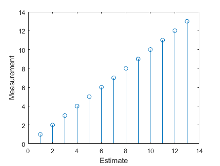
Stem plot with the x-axis labeled "Estimate" and the y-axis labeled "Measurement".

errorbar Function: Plot multiple lines with error bars at once

The errorbar function now accepts the same combinations of matrices and vectors as the plot function does. As a result, you can plot multiple lines at once rather than calling the hold function between plotting commands.
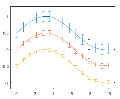
Three lines with error bars

tightPosition Function: Get the location and size of axes plotting area

Call the tightPosition function to get the location and size of the plotting area of the axes. This function is useful for aligning objects in the figure with the plotting area, particularly when you are working with polar axes, axes that display images, or other visualizations that have nondefault aspect ratios.

tilenum and tilerowcol Functions: Convert between rows and columns and tile numbers in tiled chart layouts

When working with tiled chart layouts, you can find the tile number for a specific row and column by calling the tilenum function. To find the row and column numbers that correspond to a specific tile number, use the tilerowcol function. You can also use these functions to locate the objects within the layout.

Tiled Chart Layout: Define GridSizeChangedFcn callback that executes when the grid size changes

Define the GridSizeChangedFcn callback function on a tiled chart layout. The callback function executes when the GridSize property of the layout changes. This callback is primarily useful for layouts that use the "flow" tile arrangement. For example, you can define a callback that displays the x-axis tick labels only in the bottom row of axes.

Contour Plots: Customize contour labels, colors, and transparency

Customize the appearance of a contour plot by setting these properties of the Contour object:

  • LabelFormat — Specify the formatting of the contour labels as a format operator that the compose function accepts. You can also specify a handle to a function that performs calculations when formatting the labels.

  • FaceColor and EdgeColor — Specify the fill color between contour lines with the FaceColor property, and specify the colors of the contour lines with the EdgeColor property. These new properties replace the Fill and LineColor properties from previous releases.

  • FaceAlpha and EdgeAlpha — Specify the transparency of the colors between contour lines with the FaceAlpha property, and specify the transparency of the contour lines with the EdgeAlpha property.

Two contour plots. The first plot displays contour lines against a solid light blue background with labels that include one digit after the decimal point followed by the letter m. The second plot displays the colors of the parula colormap between the contour lines. The labels in the second plot are whole numbers followed by a degree symbol and the letter C.

boxchart Function: Specify the box edge color and box median line color

The boxchart function now includes options for the box edge color and box median line color. You can specify these colors using the BoxEdgeColor and BoxMedianLineColor name-value arguments, respectively.
Four box charts with different box edge colors and median line colors

3-D Stem and Bar Plots: Expanded data type support

The stem3, bar3, and bar3h functions now support more data types. The available data types depend on the specific arguments.

These arguments can be any numeric values as well as datetime, duration, and categorical values:

  • stem3: x, y, and z (stem x and y positions and corresponding z-values)

  • bar3: y (bar positions along the y-axis)

  • bar3h: z (bar positions along the z-axis)

These arguments can be any numeric values and duration values:

  • bar3: z (bar heights)

  • bar3h: y (bar lengths)

Image Objects: Control the maximum resolution for displaying images

Control the maximum displayed resolution along the larger dimension of an image by setting the MaxRenderedResolution property when calling image or imagesc. The value affects the on-screen display, but it does not affect the image data, which is stored in the CData property of the image.

Figure Code: Generate code for figure formatting in MATLAB Online

When you edit graphics object properties for a figure in MATLAB Online using the Format tab, MATLAB generates code for the figure formatting. On the Figure tab, click the Format button to open the Format tab. Use the options in the Format tab to interactively customize properties. Then, to view, copy, or export the generated code, select Show Code in the File section of the Figure tab.

Previously, code was not generated when editing properties using the Format tab. MATLAB does not generate code when editing properties using the Property Inspector.

Plot Options: Customize figure creation, data linking, and labeling in MATLAB Online

In the Variables editor in MATLAB Online, use Plot Options in the Variable tab to customize plots and generate corresponding code in the command window. You can create a figure, link numeric data with supported charts, and generate titles, legends, and labels.

In addition, you can brush numeric data in a linked plot and create a new logical variable from selected indices. Create the logical variable by right-clicking the selection in the Variables editor or by clicking New from Selection in the Variable tab.

 Functionality being removed or changed

Legends update when you delete lines or other plot objects

Behavior change

If you delete an object from the axes, such as a Line or Scatter object, the legend updates to reflect the change regardless of whether the AutoUpdate property is set to "on" or "off".

Previously, the legend did not update when you removed objects from the axes while the AutoUpdate property was set to "off".

Plots created with tables preserve special characters in axis and legend labels

Behavior change

When you pass a table and one or more variable names to a plotting function, the axis and legend labels now display any special characters that are included in the table variable names, such as underscores. Previously, special characters were interpreted as TeX or LaTeX characters.

For example, this code creates a line plot from a table that has underscores in the variable names. In R2022b, the underscores appear in the x-axis label and the legend labels. In R2022a and earlier releases, the underscores are interpreted as subscripts.

Sample_Number = (0:10)';
Mean_AM = (2:12)';
Mean_PM = (3:13)';
t = table(Sample_Number,Mean_AM,Mean_PM);
plot(t,"Sample_Number",["Mean_AM" "Mean_PM"])
legend
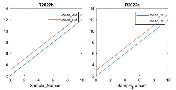
Two line plots that each have an x-axis label and a legend. The first plot was created in R2022b, and it displays the underscores in the label text. The second plot was created in R2022a, and it displays subscript characters instead of the underscores.

To display axis and legend labels with TeX or LaTeX formatting, specify the labels manually. In this case, call the xlabel and legend functions with the desired label strings.

xlabel("Sample_Number")
legend(["Mean_AM" "Mean_PM"])

Adding new plots to geographic axes does not reset basemap

Behavior change

When you plot into geographic axes by using functions such as geoplot and geoscatter, MATLAB does not reset the basemap. In R2022a and earlier releases, the basemap resets when you add new plots.

As a result, you can specify a basemap and then visualize data without using the hold function between commands. For example, this code creates a map using the streets basemap. Then it displays a scatter plot over the basemap. In R2022b, the basemap does not reset. In R2022a and earlier releases, the basemap resets to the default streets-light.

lat = [35 -22 51 39 37 42 47 -33];
lon = [139 -43 0 116 23 -71 -122 18];
 
figure
geobasemap streets
geoscatter(lat,lon,"filled")
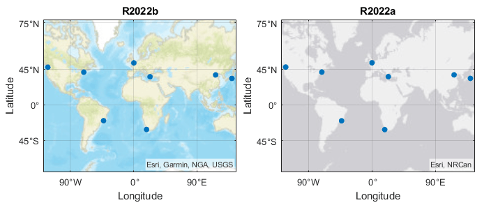
Two geographic plots. The first plot was created in R2022b, and it displays the specified streets basemap. The second plot was created in R2022a, and it displays the streets-light basemap.

This change does not affect existing code that sets the hold state to "on" between commands.

To reset the basemap when you add a new plot, use the cla reset syntax of the cla function before you create the plot. For example, to update the preceding code, use cla reset between the calls to geobasemap and geoscatter.

lat = [35 -22 51 39 37 42 47 -33];
lon = [139 -43 0 116 23 -71 -122 18];
 
figure
geobasemap streets
cla reset
geoscatter(lat,lon,"filled")

Alternatively, you can change the basemap to the default streets-light by using the geobasemap function. For more information about changing the basemap of geographic axes, see Access Basemaps for Geographic Axes and Charts.

errorbar returns error for 3-D and higher dimensional data arrays

Behavior change

The errorbar function now returns an error when you specify 3-D or higher dimensional arrays for the x-coordinates, y-coordinates, or the error bar lengths. Previously, errorbar plotted the data from the first two dimensions and silently ignored the data in the higher dimensions.

Fill and LineColor properties of Contour objects are not recommended

Still runs

Setting or getting the value of the Fill property or the LineColor property of a Contour object is not recommended. Use the FaceColor and EdgeColor properties instead. The FaceColor property provides more options for specifying colors than the Fill property does, and the EdgeColor property provides the same options as the LineColor property does.

This table shows typical usages of the Fill and LineColor properties and how to update your code to use the FaceColor and EdgeColor properties instead.

Not RecommendedRecommended

contour(peaks,"Fill",true)

contour(peaks,"FaceColor","flat")

contour(peaks,"LineColor",[0 0 0])

contour(peaks,"EdgeColor",[0 0 0])

There are no plans to remove the Fill or LineColor properties, but they are no longer listed when you call the set, get, or properties functions on the Contour object.

Some printing and exporting workflows will no longer support UI components

Still runs

These functions and menu items will no longer support printing or exporting UI components in a future release:

  • The print function

  • The saveas function

  • The hgexport function

  • The File > Save As menu item on the figure

  • The File > Export Setup menu item on the figure

  • The Edit > Copy Options menu item on the figure

To export a figure containing UI components, call the exportapp function. For example, create a simple app containing two buttons and a slider. Export the contents of the figure as a PDF file by calling the exportapp function.

% Create figure with three UI components
f = uifigure;
button1 = uibutton(f,"Position",[150 300 100 50]);
button2 = uibutton(f,"Position",[300 300 100 50]);
slider1 = uislider(f,"Position",[150 250 250 3]);

% Export the contents of the figure
exportapp(f,"myapp.pdf")

Alternatively, call the getframe function to capture the contents of the figure. Then call the imwrite function to save the content. This time, save the content as a JPEG file.

F = getframe(f);
imwrite(F.cdata,"myapp.jpg");

Exporting workflows will no longer support BMP, HDF, PBM, PCX, PGM, and PPM files

Still runs

These functions and menu items will no longer support BMP, HDF, PBM, PCX, PGM, and PPM files in a future release:

  • The print function

  • The saveas function

  • The hgexport function

  • The File > Save As menu item on the figure

  • The File > Export Setup menu item on the figure

To export graphics using one of these formats, use the imwrite function instead. For example, create a line plot, and capture the contents of the current figure using the getframe function. Then save the content as a BMP file.

plot([0 3 2 4 1]);
F = getframe(gcf);
imwrite(F.cdata,"myplot.bmp");

Some exporting workflows will no longer support PostScript (.ps) files

Still runs

These functions and menu items will no longer support creating full-page PostScript (.ps) files in a future release:

  • The print function

  • The saveas function

  • The hgexport function

  • The File > Save As menu item on the figure

  • The File > Export Setup menu item on the figure

To export graphics files, call the exportgraphics function. Specify an .eps, .pdf, or .emf file extension and set the ContentType option to "vector". This function captures content that is tightly cropped around plots, and it does not create full-page output. For example, create a plot and save the contents of the current figure as a PDF file containing vector graphics.

plot([0 3 2 4 1]);
exportgraphics(gcf,"myplot.pdf","ContentType","vector")

Alternatively, call the print function and specify an .eps, .emf, or .svg file extension. For example, create a plot and save the contents of the current figure as an EPS file.

plot([0 3 2 4 1]);
print("myplot.eps","-depsc")

The getframe function will no longer capture the figure toolbar, menu bar, or borders

Still runs

In a future release, the getframe function will no longer support capturing the figure toolbar, menu bar, or the border around the figure using the rect argument. You will still be able to define a subsection of the figure to capture, but the toolbar, menu bar, and borders will not be included.

As an alternative, you can use the exportapp function to capture the toolbar and menu bar, but not the borders.

The printopt function will be removed

Still runs

The printopt function will be removed in a future release. To configure printer defaults, use the options provided by your operating system.

App Building

ClickedFcn and DoubleClickedFcn Callbacks: Program a response to a user clicking or double-clicking a tree, check box tree, list box, table, or drop-down component

Program a response to a user clicking and double-clicking a UI component by using the ClickedFcn and DoubleClickedFcn callback properties. You can specify both of these callbacks for tree, check box tree, list box, and table UI components in App Designer and apps created using the uifigure function. You can also specify the ClickedFcn callback for drop-down components.

For more information, see the UI component properties pages:

uieditfield Function: Specify valid length and input type for edit field text

You can now specify the length and character type of valid input text for a text edit field created using the uieditfield function.

  • Use the CharacterLimits property to specify a maximum and minimum number of allowed characters.

  • Use the InputType property to restrict the allowed character types. Specify InputType as "letters", "digits", "alphanumerics", or "text".

For more information, see EditField Properties.

uiimage Function: Create an image hyperlink

To open a web address when a user clicks an image in your app, specify the URL property of the image component created using the uiimage function.

For more information, see Image Properties.

uipanel and uibuttongroup Functions: Specify container border width

In apps created using the uifigure function, use the BorderWidth property to change the border width of panels and button groups created using the uipanel and uibuttongroup functions.

For more information, see Panel Properties and ButtonGroup Properties.

uigridlayout Function: Query grid layout manager size and location

Use the Position, InnerPosition, and OuterPosition properties of a grid layout manager created using the uigridlayout function to access its size and location. These properties are read-only.

For more information, see GridLayout Properties.

uibutton and uitogglebutton Functions: Specify additional icon and icon alignment options

You can now use these additional options when adding an icon to a push button, state button, or toggle button:

  • Specify the Icon property as a predefined icon, such as "success".

  • Specify the IconAlignment property as "leftmargin" or "rightmargin" to display the icon on the far left or far right of the button, regardless of the button text location.

For more information, see Button Properties.

uitoolbar Function: Specify background color of toolbar

Specify the background color of a toolbar created using the uitoolbar function by using the BackgroundColor property. You can modify this property only in App Designer and apps created using the uifigure function.

For more information, see Toolbar Properties.

scroll Function: Programmatically scroll to specified component in container

To programmatically scroll to a component in a container or button group with the scroll function, use the syntax scroll(container,component).

isInScrollView Function: Determine if any component in a container is visible, not only direct children

When you use the isInScrollView function to determine if a UI component is visible in a scrollable container, that component can be any descendent of the scrollable container, not only a direct child. For example, you can check whether a button in a panel is visible in a scrollable UI figure.

App Designer: Add and delete callbacks more efficiently

When you select multiple components in App Designer that have a callback type in common, you can now create a single shared callback for all the selected components. For example, in an app with an edit field and a slider, you can select the two components, right-click one of them, and select Callbacks > Add ValueChangingFcn callback. App Designer creates a single new callback and assigns it to both the edit field and the slider.

You can also now more easily find callbacks in your app that are not assigned to any components. In Code View, navigate to the Callbacks tab in the Code Browser. An unassigned callback appears with a warning icon next to its name. If you do not need the callback, you can delete it by right-clicking the callback name and selecting Delete.

App Designer: Move components between tabs

To move a component from one tab to another, in Design View, drag the component and pause on the new tab. App Designer switches the selected tab to the new tab. You can then position the component in the new tab.

Graphics Support: Restore axes view and display context menu for interaction modes

In a figure created with the uifigure function or a figure in MATLAB Online, when an interaction mode is enabled, you can double-click in the axes to restore the original axes limits and view. You can also right-click to display a mode-based context menu.

For example, create a plot in a UI figure and enable the pan interaction mode.

fig = uifigure;
ax = axes(fig);
plot(ax,1:10)
pan(ax,"on");

Interactively pan the axes. Then, restore the original axes limits and view by double-clicking in the axes. You can display a mode-based context menu by right-clicking in the axes.

Previously, these workflows were supported only for figures created with the figure function.

Graphics Support: Use visual camera toolbar interface

Syntaxes of cameratoolbar that make the visual toolbar interface visible are now supported by figures created with the uifigure function. Previously, figures created with the uifigure function supported only syntaxes of the cameratoolbar function that did not directly make the toolbar visible. Now, the visual camera toolbar interface and all syntaxes are supported by figures and UI figures.

Comparison Tool: Toggle the ability to navigate only mergeable changes

When using the Comparison Tool to merge changes between two app files, you can now choose to navigate only mergeable changes. To toggle this ability, while in merge mode, click Mergeable Only in the toolstrip. If Mergeable Only is selected, when you navigate changes using the Previous and Next buttons, the tool skips changes that are not mergeable, such as changes to the noneditable code generated by App Designer. The Mergeable Only button is selected by default.

 Functionality being removed or changed

InnerPosition property of tab group returns the position excluding borders and titles

Behavior change

For apps created in App Designer and using the uifigure function, when you query the InnerPosition property of a tab group created using the uitabgroup, the property returns a different value than in the previous release. In addition, if the TabLocation is 'left' or 'bottom', when you query the Position, InnerPosition, and OuterPosition properties of a tab created using the uitab function, the properties might return different values than in the previous release.

This table describes the differences in the property values between R2022b and previous releases.

PropertyStarting in R2022bR2022a and Earlier
DescriptionImageDescriptionImage
InnerPosition of a tab groupA four-element vector of the form [left bottom width height] that represents the size and location of the tab group relative to the drawable area of its parent, excluding borders and titles of the tabs it contains

Tab group InnerPosition (blue solid line)

Tab group with tab titles on the left. A blue solid line surrounds the area of the tab group that excludes the tab titles.

A four-element vector of the form [left bottom width height] that represents the size and location of the tab group relative to the drawable area of its parent, including borders and titles of the tabs it contains

Tab group InnerPosition (blue solid line)

Tab group with tab titles on the left. A blue solid line surrounds the entire tab group, including the tab titles.

Position, InnerPosition, and OuterPosition of a tabA four-element vector of the form [left bottom width height] that represents the size and location of the tab relative to the tab group drawable area, where the tab group drawable area excludes borders and titles

Tab Position (orange dashed line) relative to tab group drawable area (blue solid line)

Tab group with tab titles on the left. A blue solid line and an orange dashed line both surround the area of the tab group that excludes the tab titles.

A four-element vector of the form [left bottom width height] that represents the size and location of the tab relative to the tab group drawable area, where the tab group drawable area includes borders and titles

Tab Position (orange dashed line) relative to tab group drawable area (blue solid line)

Tab group with tab titles on the left. A blue solid line surrounds the entire tab group, including the tab titles. An orange dashed line surrounds the area of the tab group that excludes the tab titles, and is offset on the left from the blue solid line.

If you notice changes in your app layout, consider updating your code in this way:

  • Tab group InnerPosition — Replace references to the tab group InnerPosition property with the tab group Position property to use the size and location of the tab group including the borders and tab titles.

  • Tab Position, InnerPosition, and OuterPosition — Replace references to the first two elements of the position vector to instead use the space taken up on the left or bottom by the tab titles. For example, if your app contains a tab group with a TabLocation value of 'left' and you reference the Position property of a tab in that tab group, replace that reference with the horizontal distance between the tab group border and the tab drawable area.

Table Extent property will return the default table UI component width and height

Behavior change in future release

In a future release, when you query the Extent property of a table UI component created using the uitable function in a figure-based app, the property will always return [0 0 300 300]. The third and fourth elements of the vector represent the default table width and height. Currently, querying Extent returns a vector where the third and fourth elements represent the width and height of the rectangle outlining the table area, estimated using the table data, row heights, and column widths. If you use the Extent property to specify the position of UI components in your app, the table UI component might have a different size or the layout of your app might appear shifted.

Consider updating your code to remove references to the table Extent property by using one of these alternatives:

  • Lay out the table and other UI components by manually specifying the Position property.

  • Transition your figure-based app to use uifigure, and use a grid layout manager with a row height or column width of 'fit' to automatically scale your app layout based on the size of the table with its data. For more information, see Update figure -Based Apps to Use uifigure.

Performance

prctile, quantile, and iqr Functions: Improved performance with small input data

The prctile, quantile, and iqr functions show improved performance due to faster input parsing. The performance improvement is most significant when input parsing is a greater portion of the computation time. This situation occurs when:

  • The size of the input data is small.

  • The number of percentages or cumulative probabilities is small.

  • Computation is along the default operating dimension.

For example, this code calculates four percentiles for a 3000-element matrix. The code is about 5x faster than in the previous release.

function timingPrctile
A = rand(300,10);
for k = 1:3e3
  P = prctile(A,[20 40 60 80]);
end
end

The approximate execution times are:

R2022a: 1.0 s

R2022b: 0.2 s

The code was timed on a Windows 10, Intel Xeon CPU E5-1650 v4 @ 3.60 GHz test system using the timeit function.

timeit(@timingPrctile)

mldivide and pagemldivide Functions: Improved performance with small matrices

The mldivide and pagemldivide functions show improved performance when solving linear systems A*x = b with a small coefficient matrix A. The performance improvement applies to real matrices that are 16-by-16 or smaller, and complex matrices that are 8-by-8 or smaller.

  • Using mldivide, this code solves a linear system specified by a real 12-by-12 matrix. The code is about 1.7x faster than in the previous release.

    function mldividePerf
    A = rand(12);
    for k = 1:1e5
        x = A\A;
    end
    end

    The approximate execution times are:

    R2022a: 0.72 s

    R2022b: 0.42 s

  • Using pagemldivide, this code solves three triangular linear systems specified by an 11-by-11-by-3 array. The code is about 2.2x faster than in the previous release.

    function pagemldividePerf
    a = triu(rand(11));
    A = cat(3,a,a,a);
    for k = 1:1e5
        x = pagemldivide(A,A);
    end
    end
    

    The approximate execution times are:

    R2022a: 0.65 s

    R2022b: 0.30 s

In both cases, the code was timed on a Windows 10, Intel Xeon CPU W-2133 @ 3.60 GHz test system using the timeit function:

timeit(@mldividePerf)
timeit(@pagemldividePerf)

conv, conv2, and convn Functions: Improved performance when convolving two vectors, matrices, and arrays

The conv, conv2, and convn functions show improved performance when convolving two vectors, matrices, and arrays for almost all input sizes.

  • Using conv, this code convolves a 1,000,000-by-1 vector and a 10,000-by-1 vector. The code is about 3x faster than in the previous release.

    function timingTest
    rng default;
    u = randn(1000000,1);
    v = randn(10000,1);
    tic
    w = conv(u,v);
    toc
    end

    The approximate execution times are:

    R2022a: 0.40 s

    R2022b: 0.13 s

  • Using conv2, this code convolves a 512-by-512 matrix and a 256-by-256 matrix. The code is about 4x faster than in the previous release.

    function timingTest
    rng default;
    A = randn(512);
    B = randn(256);
    tic
    C = conv2(A,B);
    toc
    end

    The approximate execution times are:

    R2022a: 0.97 s

    R2022b: 0.24 s

  • Using convn, this code convolves a 128-by-64-by-32 array and a 64-by-32-by-16 array. The code is about 4.9x faster than in the previous release.

    function timingTest
    rng default;
    A = randn(128,64,32);
    B = randn(64,32,16);
    tic
    C = convn(A,B);
    toc
    end

    The approximate execution times are:

    R2022a: 1.08 s

    R2022b: 0.22 s

All of the code was timed on a Windows 10, Intel Xeon CPU E5-1650 v4 @ 3.60 GHz test system by calling the timingTest function in each case.

Tall Arrays: Improved performance when indexing tall arrays backed by parquetDatastore

Tall arrays backed by parquetDatastore show improved performance with row-indexing operations. The performance improvement arises from the use of predicate pushdown to reduce the amount of data that is imported into MATLAB. So, the improved performance is most noticeable with data that has a large number of rows compared to the number of rows returned by the indexing operation. The improvement gets better as the number of rows being filtered increases.

For example, this code creates a tall array backed by a Parquet datastore for the airlinesmall.parquet file, and then performs row indexing to extract rows that meet several specified conditions. The operation returns 10 rows out of 1.2 million and executes about 2.3x faster than in the previous release.

function parquetPerf
mapreducer(0)
pds = parquetDatastore("airlinesmall.parquet");
pds.Files = repelem(pds.Files,10);
T = tall(pds);
conditions = T.DepDelay >= seconds(10) & T.DepDelay <= seconds(80) ...
    & T.UniqueCarrier == "AA" ...
    & T.DepTime >= datetime(2000,1,1) & T.DepTime < datetime(2000,1,7);

idx_rows = T(conditions,:);
g = gather(idx_rows);
end

The approximate execution times are:

R2022a: 8.0 s

R2022b: 3.5 s

The code was timed on a Windows 10, Intel Xeon CPU W-2133 @ 3.60 GHz test system using the timeit function:

timeit(@parquetPerf)

App Building: Improved app startup performance

Apps created in App Designer and using the uifigure function start up faster in R2022b than in R2022a. The improvement is more noticeable for apps with many UI components and apps that use a grid layout manager. The startup performance is faster both the first time you run your app during a MATLAB session and in subsequent times.

For example, this code creates an app with 1000 edit field components. The code is about 1.6x faster than in the previous release.

function timingApp
fig = uifigure;
gl = uigridlayout(fig,Scrollable="on");
gl.RowHeight = repmat({'fit'},1,100);
gl.ColumnWidth = repmat({'fit'},1,10);

for k = 1:1000
    uieditfield(gl);
end
drawnow
end

The approximate execution times are:

R2022a: 17.3 s

R2022b: 10.6 s

The code was timed on a Windows 10, Intel Xeon CPU E5-1650 v4 @ 3.60 GHz test system by running the timingApp function and measuring the time it takes for the edit fields to appear in the UI figure window.

 App Building: Improved startup performance for apps with multiple tabs

In addition to the overall app startup performance improvement in R2022b, apps that contain multiple tabs show an even greater startup performance improvement. The reason is that MATLAB prioritizes creating the content in the visible tab over non-visible content when the app first runs. This improvement is more noticeable for apps with a large number of UI components in unselected tabs. The particular performance improvement that you see depends on the app layout and UI component types.

For example, this code creates a tab group with five tabs, each containing 200 edit field components. The code is about 1.9x faster than in the previous release.

function timingTabApp
fig = uifigure;
tg = uitabgroup(fig);

for k1 = 1:5
    t = uitab(tg);
    gl = uigridlayout(t,Scrollable="on");
    gl.RowHeight = repmat({'fit'},1,20);
    gl.ColumnWidth = repmat({'fit'},1,10);
    for k2 = 1:200
        uieditfield(gl);
    end
end
drawnow
end

The approximate execution times are:

R2022a: 11.8 s

R2022b: 6.3 s

The code was timed on a Windows 10, Intel Xeon CPU E5-1650 v4 @ 3.60 GHz test system by running the timingTabApp function and measuring the time it takes for the components to appear in the UI figure window.

If you have an app with many UI components, consider updating your app layout to take advantage of this improvement. For more information, see Improve App Startup Time.

 Compatibility Considerations

When an app user switches to a new tab for the first time after running an app, the interaction might take more time than in previous releases. The reason is that MATLAB might create some content in the tab only after the user selects the tab. If the user later switches to the same tab again, the interaction does not take the additional time.

Plots in Apps: Improved responsiveness when interacting with large images

Interactions with large images are more performant within apps and within figures created with the uifigure function. The improvement is noticeable for images with at least 3000 pixels along one dimension. In particular, these interactions are more responsive in R2022b than in R2022a:

  • Zooming out — The image updates immediately after you zoom out of an image. Previously, there was a delay before the image updated.

  • Panning — The image updates as you are panning within an image. Previously, the image updated after you finished panning (for example, after releasing the mouse).

For example, if you run this code on a Windows 10, Intel Xeon CPU W-2133 @ 3.60 GHz test system with a modern graphics card, and then zoom into the resulting image and pan around, the image updates immediately as you interact.

imdata = imread("peppers.png");
imdata2 = repmat(imdata,8,8,1);
f = uifigure;
ax = axes(f);
image(ax,imdata2)
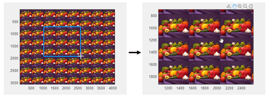
Two figures in succession: One figure shows the crosshair selection cursor selecting part of an image to zoom into. The second figure shows the hand-shaped cursor panning within the image.

Plots in Apps: Ticks and grid lines update as you pan

Axes ticks and grid lines update immediately as you pan within many types of Cartesian plots that are displayed in apps. Previously, the ticks and grid lines updated after you released the mouse. Now, the ticks update immediately for most plots that meet all of these conditions:

  • They are in 2-D Cartesian space

  • They display numeric data on a linear scale

  • They have the default tick values and labels

  • They have the default axis locations

Grid lines update immediately under the same conditions, but you can see the improvement in 3-D views in addition to 2-D views.

For example, if you run this code on a Windows 10, Intel Xeon CPU W-2133 @ 3.60 GHz test system and then pan within the axes, the ticks and the grid lines update immediately as you pan.

f = uifigure;
ax = uiaxes(f);
x = 1:50;
y = rand(1,50);
plot(ax,x,y);
ax.XLim = [20,30];
grid(ax,"on")
Line plot with ticks and grid lines, and a hand shaped cursor for panning around the plot

Plots in Apps: Improved performance and smaller PDF files when exporting complex plots

The exportgraphics function has improved performance and creates a smaller file when you export a complex graphic as a PDF containing vector graphics. To observe the improvement, the plot must be displayed in an app or in a figure created with the uifigure function. For example, this code creates a figure containing a complex contour plot. Then it calls the exportgraphics function to export the plot as a PDF containing vector graphics content. The exportgraphics function executes about 2.1x faster, and the file size is about 23% smaller than in the previous release.

function myapp
f = uifigure;
ax = uiaxes(f);
x = linspace(-250*pi,250*pi);
y = linspace(0,500*pi);
[X,Y] = meshgrid(x,y);
Z = sin(X)+cos(Y);
contour(ax,X,Y,Z,50)
tic
exportgraphics(ax,"mycontours.pdf","contentType","vector")
toc
end
Contour plot of Z = sin(X)+cos(Y)

The approximate execution times (and file sizes) are:

R2022a: 16.3 s (3.45 MB)

R2022b: 7.7 s (2.66 MB)

The code was timed on a Windows 10, Intel Xeon CPU E5-2660 @ 2.20 GHz test system by calling the myapp function:

myapp

Tiled Chart Layouts: Improved performance for flow layouts with spanned axes

Tiled chart layouts that have the "flow" tile arrangement and axes that span several tiles are more performant when they update. Layouts update when you make changes that affect the arrangement of the tiles, including:

  • Adding new axes

  • Resizing the figure

  • Customizing the appearance of the axes by setting axes properties

The performance improvement is more significant when there are axes that span many tiles. For example, this code is about 1.4x faster than in the previous release.

function mylayout
t = tiledlayout("flow");
nexttile(t,[20 15])
nexttile(t,[20 15])
nexttile(t,[10 30])
nexttile(t,[10 30])
nexttile(t,[10 30])
drawnow
end
Five axes in a tiled chart layout that span several rows and columns

The approximate execution times are:

R2022a: 0.1082 s

R2022b: 0.0788 s

The code was timed on a Windows 10, Intel Xeon CPU W-2133 @ 3.60 GHz test system using the timeit function:

timeit(@mylayout)

ArrayDatastore Object: Improved performance when reading data using readall

The readall function shows improved performance when reading data from an ArrayDatastore object that has an OutputType property set to "same". The readall function increases performance by removing unnecessary data copies. For example, this code is significantly faster than in the previous release:

function t = timingTest
    data = parquetread("airlinesmall.parquet");
    arrds = arrayDatastore(data,OutputType="same");
    tic;
    t = readall(arrds);
    toc;
end

The approximate execution times are:

R2022a: 1584.36 seconds

R2022b: 0.12 seconds

The code was timed on a Windows 10, Intel Xeon (R) W-2133 @ 3.60 GHz test system by calling the timingTest function.

ArrayDatastore Object: Improved performance when specifying number of rows to read

The read function shows improved performance when reading data from an ArrayDatastore object that has an OutputType property set to "same" and a value specified for the ReadSize property. The performance improvement increases as the ReadSize value gets larger. For example, this code is about 4.5x faster than in the previous release:

function c = timingTest
    data2 = parquetread("outages.parquet");
    arrds = arrayDatastore(data2, OutputType="same",ReadSize=100);
 
    index = 1;
    c = cell([ceil(numpartitions(arrds)/100) 1]);
    
    tic;
    while hasdata(arrds)
        c{index} = read(arrds);
        index = index + 1;
    end
    toc;
end

The approximate execution times are:

R2022a: 0.90 seconds

R2022b: 0.20 seconds

The code was timed on a Windows 10, Intel Xeon (R) W-2133 @ 3.60 GHz test system by calling the timingTest function.

parquetread Function: Improved performance reading string data from Parquet files

The parquetread function shows improved performance when reading string data from a Parquet file. For example, this code is about 1.23x faster than in the previous release:

function t = timingTest
    info = parquetinfo("airlinesmall.parquet");
    varNames = info.VariableNames(info.VariableTypes == "string");
    
    tic;
    for i = 1:20
        t = parquetread("airlinesmall.parquet",SelectedVariableNames=varNames);
    end
    toc;
end

The approximate execution times are:

R2022a: 4.93 seconds

R2022b: 4.00 seconds

The code was timed on a Windows 10, Intel Xeon (R) W-2133 @ 3.60 GHz test system by calling the timingTest function.

parquetDatastore Function: Improved performance when creating datastore with large number of Parquet files

The parquetDatastore function shows improved performance when creating a datastore with a large number of Parquet files. For example, this code runs about 2.5x faster than in the previous release:

function pds = timingTest
    filenames = repmat("airlinesmall.parquet",1000,1);
    
    tic;
    for i = 1:20
        pds = parquetDatastore(filenames);
    end
    toc;
end

The approximate execution times are:

R2022a: 105.31 seconds

R2022b: 42.03 seconds

The code was timed on a Windows 10, Intel Xeon (R) W-2133 @ 3.60 GHz test system by calling the timingTest function.

Workspace Browser: Improved performance of variable-deletion dialog boxes in MATLAB Online

In MATLAB Online, confirmation dialog boxes for interactively deleting variables from the MATLAB Workspace show improved performance. The delay between selecting Delete or Clear Workspace for variables in the Workspace browser and the confirmation dialog box appearing is reduced.

For example, on a Windows 10, Intel Xeon CPU E5-1650 v4 @ 3.60 GHz test system, when you right-click a single variable in the workspace and select Delete, the confirmation dialog box appears more quickly in R2022b than in R2022a.

Variables Editor and Live Editor: Improved speed of data display when scrolling in MATLAB Online

In MATLAB Online, for variables in the Variables editor or in the generated output of the Live Editor, the performance of vertical and horizontal scrolling is improved. Improved infinite scrolling queries data more efficiently, so data appears more quickly after scrolling in R2022b than in the previous release.

For example, on a Windows 10, Intel Xeon CPU E5-1650 v4 @ 3.60 GHz test system, when you scroll through a table with 3000 rows, the displayed data renders more quickly in R2022b than in R2022a.

lookfor Function: Improved performance when searching

The lookfor function shows improved performance when searching for keywords.

For example, if you use the lookfor function to search for the keyword inverse in the summary line of all the references pages in the MathWorks documentation, search results appear about 36x faster than in the previous release.

function timingTest
lookfor inverse
end

The approximate execution times are:

R2022a: 6.8885 s

R2022b: 0.1909 s

Similarly, if you use the lookfor function to search for the keyword inverse in the summary line and the Syntax, Description, Input Arguments, Output Arguments, and See Also sections of all the reference pages in the MathWorks documentation, search results appear about 5x faster than in the previous release.

function timingTest
lookfor inverse -all
end

The approximate execution times are:

R2022a: 9.5596 s

R2022b: 1.7926 s

The code was timed on a Windows 10, Intel Xeon CPU W-2133 @ 3.60 GHz test system using the timeit function.

timeit(@timingTest)

Software Development Tools

Build Tool: Create and run software-build tasks

You can use a standard programming interface to create and run software-build tasks in a uniform and efficient way. For example, you can create tasks that identify code issues, run tests, and package a toolbox in a single build file in your project root folder, and then invoke the build tool to run these tasks. For more information, see Overview of MATLAB Build Tool.

Dependency Analyzer: New warnings to identify problems

When you run a dependency analysis, the Dependency Analyzer now warns about files that contain a syntax error. See Investigate and Resolve Problems.

Project API: Extract project from archive

You can now extract a project from an archive by using matlab.project.extractProject.

Source Control in MATLAB Online: Manage Git branches and repositories

You can now manage Git branches and repositories in MATLAB Online:

  • Create, switch, merge, and delete branches.

  • Find and compare commits.

  • Create branches from a tag or a revision.

  • View the history of a Git repository.

  • Manage multiple Git repositories at once.

Unit Testing Framework: Add methods and properties to test classes interactively

You can add code to your test classes interactively. With a file defining your class-based test in the Editor, go to the Editor tab and in the Test section, choose whether to add a method or parameterization property at the test level, method-setup level, or class-setup level. For more information, see Insert Test Code Using Editor.

Unit Testing Framework: Specify action to take against invalid test files

You can specify whether the framework issues a warning or throws an error when it encounters an invalid test file in a folder or package. To specify the action, use the InvalidFileFoundAction name-value argument. For example, s = testsuite(pwd,InvalidFileFoundAction="error") creates a test suite only if the current folder does not contain invalid test files and throws an error otherwise. Examples of invalid test files include a test file that contains syntax errors, a function-based test file that is missing local functions, and a file with a Test method that is passed an undefined parameterization property.

You can specify the InvalidFileFoundAction name-value argument for these methods and functions:

 Unit Testing Framework: Generate descriptive test parameter names using cell arrays

Starting in R2022b, when you assign a nonempty cell array to a parameterization property, the testing framework generates parameter names from the elements of the cell array by taking into account their values, types, and dimensions. In previous releases, if the property value is a cell array of character vectors, the framework generates parameter names from the values in the cell array. Otherwise, the framework specifies parameter names as value1, value2, …, valueN.

For example, create a test class with parameterization properties that are set using cell arrays.

classdef SampleTest < matlab.unittest.TestCase
    properties (TestParameter)
        numericArray = {int16(1),single(zeros(1,4)),magic(3)};
        functionHandle = {@false,@() size([])};
    end
    methods (Test)
        function test1(testCase,numericArray)
            testCase.verifyNotEmpty(numericArray)
        end
        function test2(testCase,functionHandle)
            testCase.verifyWarningFree(functionHandle)
        end
    end
end

Create a test suite from the class and return the names of the suite elements.

R2022a and EarlierStarting in R2022b
suite = testsuite("SampleTest");
{suite.Name}'
ans =

  5×1 cell array

    {'SampleTest/test1(numericArray=value1)'  }
    {'SampleTest/test1(numericArray=value2)'  }
    {'SampleTest/test1(numericArray=value3)'  }
    {'SampleTest/test2(functionHandle=value1)'}
    {'SampleTest/test2(functionHandle=value2)'}
suite = testsuite("SampleTest");
{suite.Name}'
ans =

  5×1 cell array

    {'SampleTest/test1(numericArray=int16_1)'          }
    {'SampleTest/test1(numericArray=1x4_single)'       }
    {'SampleTest/test1(numericArray=3x3_double)'       }
    {'SampleTest/test2(functionHandle=@false)'         }
    {'SampleTest/test2(functionHandle=function_handle)'}
 Compatibility Considerations

If you use parameter names in your code to create or filter test suites, use the descriptive parameter names. This table shows an example of how to update code that filters the test suite created from the SampleTest class.

BeforeAfter
import matlab.unittest.selectors.HasParameter
s = ~HasParameter("Property","numericArray","Name","value1");
suite2 = selectIf(suite,s);
import matlab.unittest.selectors.HasParameter
s = ~HasParameter("Property","numericArray","Name","int16_1");
suite2 = selectIf(suite,s);

Unit Testing Framework: Compare dictionaries in tests

The IsEqualTo constraint supports MATLAB dictionaries. The constraint treats two dictionaries as equal if they have the same keys and the values assigned to corresponding keys also satisfy the constraint. For example, this test passes.

import matlab.unittest.TestCase
import matlab.unittest.constraints.IsEqualTo
import matlab.unittest.constraints.DictionaryComparator
import matlab.unittest.constraints.NumericComparator

testCase = TestCase.forInteractiveUse;
actual = dictionary(["key1" "key2"],[1 2]);
expected = dictionary("key1",1,"key2",2);
testCase.verifyThat(actual,IsEqualTo(expected, ...
    Using=DictionaryComparator(NumericComparator)))

To override how dictionaries are compared by IsEqualTo, use the matlab.unittest.constraints.DictionaryComparator class.

 Functionality being removed or changed

pack function has been removed

Errors

The pack function has been removed. There is no replacement for this function because you do not need to use it on a 64-bit system. For more information about strategies for reducing memory usage, see Strategies for Efficient Use of Memory and Resolve “Out of Memory” Errors.

Interactively running a test class requires the class definition file to explicitly use framework-specific data

Behavior change

When you open a class-based test file in the MATLAB Editor, you can interactively run the tests in the file only if the test class explicitly subclasses a TestCase class, uses framework-specific attributes to specify test content, or both. In previous releases, the testing framework tries to examine the class hierarchy whenever it cannot determine if a class definition file contains a test class. This change of behavior prevents checks that might take a long time to complete.

For example, consider an abstract test class defined to test if a function supports implicit expansion of a scalar input.

classdef ScalarExpansionTest < matlab.unittest.TestCase
    properties (Abstract)
        FcnHandle
    end
    methods (Test)
        function supportsScalarExpansion(testCase)
            fcn = testCase.FcnHandle;
            result = fcn(1,1:5);
            testCase.verifySize(result,[1 5], ...
                "Result must be a 1-by-5 vector.");
        end
    end
end

To test scalar expansion with a specific function interactively, make sure to specify framework-specific data when you create a concrete test class from ScalarExpansionTest. If your test class does not require any framework-specific attributes (such as Test, TestParameter, and TestTags), consider deriving it explicitly from matlab.unittest.TestCase. In this example, you can run PlusTest interactively because the framework can determine the class type using the contents of the class definition file.

classdef PlusTest < ScalarExpansionTest & matlab.unittest.TestCase
    properties
        FcnHandle = @plus;
    end
end

External Language Interfaces

.NET Interface: Support for .NET 5 and .NET Core

On Microsoft Windows platforms, MATLAB supports loading libraries compiled for .NET 5 and higher and for .NET Core, in addition to existing support for the Microsoft .NET Framework. To select a .NET environment, use the dotnetenv function. For more information, see Selecting .NET Core in MATLAB.

.NET Engine API: Call MATLAB from .NET applications

The MATLAB Engine API for .NET provides an interface between .NET programming languages and MATLAB. This API enables programs to launch MATLAB, evaluate MATLAB functions with arguments, and exchange data between MATLAB and .NET programs. For more information, see Call MATLAB from .NET and MathWorks.MATLAB.Engine.MATLABEngine.

If you write code that calls MATLAB as a COM Automation server using the MATLAB COM Automation Server Interface, consider using the MATLAB Engine API for .NET instead.

Publish C++ Interface: Support for char* output as nullTerminated string

You can specify a nullTerminated string for char* and const char* return types. For details, see the C++ Return Type table with the C++ to MATLAB data type mapping for C++ char* and char[] Types.

Call MATLAB from C++: Use MATLAB enumeration classes in strongly-typed interface

To generate C++ code from a MATLAB enumeration, use the Classes name-value argument with the matlab.engine.typedinterface.generateCPP function. For example, to create a header file InterfaceCode.hpp from a MATLAB enumeration class MyColorEnum with a function printMyText, type:

matlab.engine.typedinterface.generateCPP("InterfaceCode.hpp",Classes="MyColorEnum",Functions="printMyText")

Python Interface: Display keyword (key-value pair) arguments created by pyargs

The pyargs function displays keyword (key-value pair) arguments.

pyargs(A=1,B=2)
ans = 

  'pyargs' with pairs:

    A: 1
    B: 2

Python Interface: Convert scalar logical and numeric Python types to MATLAB types

You can convert Python data types py.int, py.long, py.float, and py.bool to MATLAB types using these MATLAB functions:

  • double

  • single

  • int8

  • uint8

  • int16

  • uint16

  • int32

  • uint32

  • int64

  • uint64

  • logical

For information about conversion functions, see MATLAB to Python Data Type Mapping.

Python Engine: Pass NumPy arrays directly to MATLAB functions

Calls to MATLAB functions from Python engine applications accept any object that implements the Python buffer protocol, like NumPy arrays, as an input argument.

For example, this code calls the built-in MATLAB function sum with a NumPy ndarray buf as input.

import matlab.engine
import numpy
eng = matlab.engine.start_matlab()
buf = numpy.array([[1, 2, 3], [4, 5, 6]], dtype='uint16')

# Supported in R2022a and earlier: must initialize a matlab.uint16 from
# the numpy array and pass it to the function
array_as_matlab_uint16 = matlab.uint16(buf)
res = eng.sum(array_as_matlab_uint16, 1, 'native')
print(res)

# Supported as of R2022b: can pass the numpy array
# directly to the function
res = eng.sum(buf, 1, 'native')
print(res)

For information about using the MATLAB Engine API for Python, see Call MATLAB from Python.

Python Engine: Install MATLAB Engine API with pip Command

You can use the pip command to install the MATLAB Engine API. For more information, see Install MATLAB Engine API for Python.

Python: Support for Version 3.10

MATLAB now supports CPython version 3.10, in addition to existing support for versions 2.7, 3.8, and 3.9. For more information, see Versions of Python Compatible with MATLAB Products by Release.

 Functionality being removed or changed

C++ library definition file has .m file extension

Behavior change

The clibgen.generateLibraryDefinition function creates library definition files with .m file extensions. The function no longer creates a file with the .mlx file extension. You can continue to modify and build existing library definition files with the .mlx file extension.

For information about editing the library definition file, see How to Complete Definitions in Library Definition File. While following the instructions, note that when you uncomment the code defining a function, do not uncomment the first two lines in the code section. These comments contain the section title and the C++ signature help.

Python: Version 2.7 support will be discontinued in a future release

Behavior change in future release

Support for Python version 2.7 will be discontinued in a future release.

To ensure continued support for interacting between Python and MATLAB, consider upgrading to a supported version of Python. For supported version information, see Versions of Python Compatible with MATLAB Products by Release.

Hardware Support

Upload Libraries and Configure Pins for I2C, SPI, and Serial Communication Using the Arduino Explorer App

The Arduino Explorer app, which was introduced in R2021b release of MATLAB Support Package for Arduino Hardware, now supports selecting and uploading the required libraries for the initial setup of the Arduino board. The modified app also allows you to configure pins on the Arduino board for I2C, SPI, and Serial communication, and plot the values. You can also add decode logic on the read values and view the values in the Log panel of the app.

 Support for servo and rotary encoder peripherals connected to Arduino-compatible ESP32 boards

In addition to the existing support for communicating with I2C, SPI and serial peripherals connected to Arduino-compatible ESP32 board, the MATLAB Support Package for Arduino Hardware now supports communicating with servo and rotary encoder peripherals connected to the board.

R2022a

New Features, Bug Fixes, Compatibility Considerations

Environment

Themes in MATLAB Online: Change the colors of the MATLAB desktop by selecting a dark or light theme

In MATLAB Online, you can change the colors of the MATLAB desktop using themes.

For example, to select a dark theme, on the Home tab, in the Environment section, click Preferences. Select MATLAB > Appearance and set the Theme to Dark.
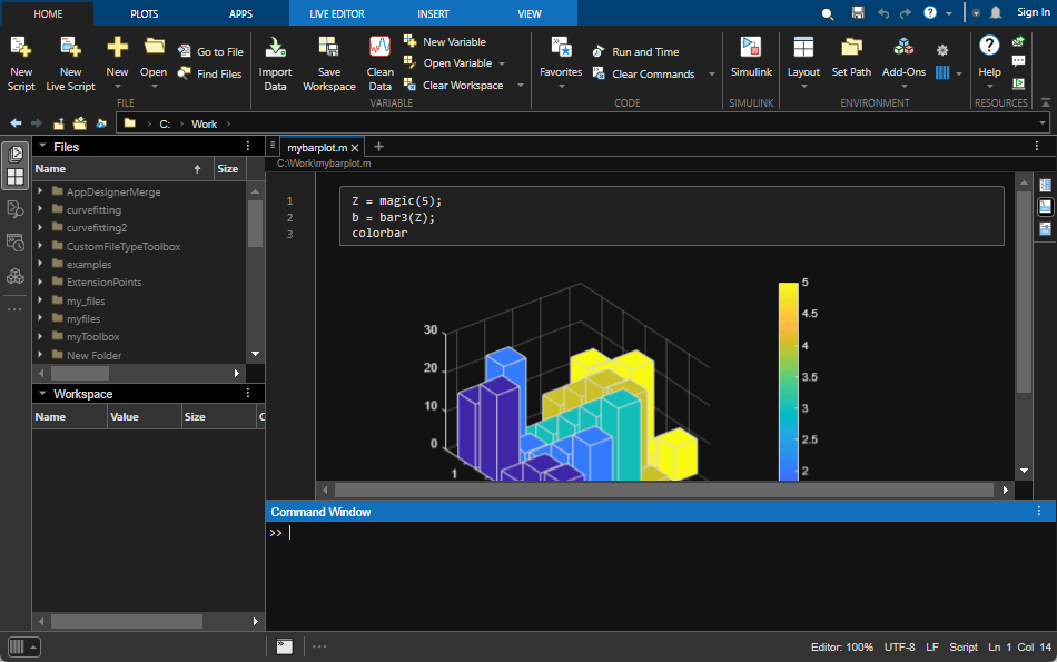
MATLAB desktop with all panels displayed with a dark background and light text

To further customize the colors of the MATLAB desktop, select MATLAB > Appearance > Colors. Then, change the colors in the Desktop tool colors, MATLAB syntax highlighting colors, and MATLAB output colors sections.

As part of this change, icons in the MATLAB Online desktop have an improved visual appearance.

For more information about changing the colors of the MATLAB desktop, see Change Desktop Colors.

Live Editor Colors: Change the text and background colors of live scripts and functions

You can change the text and background colors in the Live Editor by changing the MATLAB desktop tool colors.

To change the text and background colors:

  1. On the Home tab, in the Environment section, click Preferences.

  2. Select MATLAB > Colors

    In MATLAB Online, select MATLAB > Appearance > Colors.

  3. In the Desktop tool colors section, clear the Use system colors check box.

    In MATLAB Online, the Use system colors check box is not available and this step can be skipped.

  4. Use the Text and Background fields to change the colors. For example, select white for the text color and black for the background color.

The Live Editor automatically selects colors for titles and headings based on the selected background color. To further customize the colors of titles and headings, use settings. For more information, see matlab.fonts Settings.

Live Editor Hyperlinks: Insert hyperlinks to specific locations in separate live scripts or live functions

Use hyperlinks to navigate to a location in a separate, existing live script or function. To insert a hyperlink, select the text to link in the current file, go to the Insert tab, and click Hyperlink. Edit your display text (optional), select Location in existing document, and enter or browse for the file path. Then, select a location in the document preview that displays on the right.

For more information about inserting hyperlinks, see Format Text in the Live Editor.

Live Editor Export: Export live scripts and functions programmatically using the export function

Use the export function to programmatically export live scripts and functions to a standard format. Available formats include PDF, Microsoft Word, HTML, and LaTeX.

For example, to export the live script homework1.mlx as HTML, type:

export("homework1.mlx","homework1.html")

Live Editor Accessibility: Interact with output in live scripts using the keyboard

You can now use keyboard shortcuts to interact with output in live scripts when output is on the right. To move focus from the code to the output display panel, press Ctrl+Shift+O. On macOS, press Option+Command+O. To activate an output, press Enter. Once an output is activated, you can scroll text using the arrow keys, navigate through hyperlinks and buttons using the Tab key, and open the context menu by pressing Shift+F10.

Live Editor Tasks: View and interact with tasks when code is hidden

When you hide code in a live script, the Live Editor now displays Live Editor tasks along with formatted text, labeled controls, and output.

To hide code, select the Hide Code button to the right of the live script or in the View tab. Alternatively, if you are using the export function, you can hide the code using the HideCode name-value argument.

If a Live Editor task is configured to show only code and no controls, then the task does not display when you hide code.

Component Browser: Reorder children in App Designer or the Property Inspector

You can now drag one or more Axes object children, Group object children, or Transform object children sharing the same parent to reorder them in the Component Browser in App Designer or the Property Inspector for figures.

When reordering children, use visual feedback for allowed moves. You can undo and redo the reordering of the children with Undo or Redo or the corresponding keyboard shortcuts.

Editor Python Support: View and edit Python files with syntax highlighting, auto-indenting, and delimiter matching

The Editor now displays Python files with syntax highlighting for keywords, strings, comments, and errors. In addition, the Editor auto-indents Python files and indicates matched and mismatched delimiters such as parentheses, brackets, and braces.

Find and Replace Dialog Box: Search text in the Editor and Live Editor using regular expressions

You can use a subset of regular expressions to search for text that matches a pattern in an open file in the Editor or Live Editor. To search using a regular expression, on the Editor or Live Editor tab, in the Navigate section, click Find. Then, in the find and replace dialog box, enter a regular expression, and select the Regular Expression button .

For example, to find all the words in a file that contain the letter x, enter the expression \w*x\w* and select the Regular Expression button .

Find and replace dialog box with the Regular Expression button selected and the expression \w*x\w* in the Find text field

For more information, see Find and Replace Text in Files and Go to Location.

Profiler: Access the Profiler from the Apps tab

The MATLAB Profiler is now available as an app and can be found in the MATLAB section of the apps gallery in the Apps tab.

You can still access the Profiler from the Home tab, in the Code section, by clicking the Run and Time button, or programmatically using the profile function.

Internationalization: UTF-8 system encoding on Windows platforms

MATLAB now uses UTF-8 as its system encoding on Windows, completing the adoption of Unicode across all supported platforms. MATLAB has used UTF-8 as the default encoding for MATLAB files and file I/O since R2020a.

If you see garbled characters on a Windows Server® 2019 platform, then enable the Beta: Use Unicode UTF-8 for worldwide language support option in Region Settings.

Installation Settings: Configure persistent settings for MATLAB installations

Installation-level settings provide a new layer of MATLAB configuration that lies between factory settings and personal settings. Installation settings override the factory settings for all users of a given MATLAB installation, and they are persistent across sessions.

In previous versions of MATLAB, if administrators wanted to limit RAM usage for a set of MATLAB users by lowering the ArraySizeLimit, they had to create and distribute a script to change the personal setting for each individual user. Starting in R2022a, the administrator can apply the change to all users of their MATLAB installation using the installation setting for ArraySizeLimit.

Access installation-level settings using the new InstallationValue property of the Setting object. Verify and clear installation settings with two new object functions, hasInstallationValue and clearInstallationValue, respectively.

Comparison Tool: Save results as HTML report

You can now use the Comparison Tool to publish text comparison results in an HTML report. For more details, see Compare Text Files.

Comparison Tool: Compare folders in MATLAB Online

Starting in R2022a, you can compare folders and zip files in MATLAB Online.

You can access the comparison tool from:

  • The MATLAB Current Folder browser context menu

  • The Current Project browser context menu

  • The MATLAB Command Window using the visdiff function

MATLAB Drive: macOS 10.15 Catalina will no longer receive updates to MATLAB Drive Connector (April 2022)

After this release, macOS 10.15 Catalina will no longer receive updates to MATLAB Drive Connector.

Installing later versions of MATLAB Drive Connector on macOS 10.15 Catalina will not be supported. In addition, the Connector will not automatically update to a later version when one becomes available.

 Functionality being removed or changed

Live Editor figure size is bounded upon saving

Behavior change

When opening a saved live script, existing images in the output have a maximum size equivalent to the figure size upon saving. To adjust the size past this maximum limit, you can run the live script and increase the figure size.

Language and Programming

Class Introspection: Description and DetailedDescription properties of metaclasses contain text from code comments

The Description and DetailedDescription properties of these metaclasses pull content from code comments:

For user-defined classes with appropriately placed code comments, the Description and DetailedDescription properties of the metaclasses are populated with text pulled from those comments. For more information on how to use code comments to store custom help text for user-defined classes, see Custom Help Text.

Class Introspection: Access class aliases from meta.class instance

The aliases of a class are stored in the new Aliases property of meta.class. For more information on class aliasing, see Creating and Managing Class Aliases.

Background Pool: See futures in the background

Starting in R2022a, you can query all queued and running futures in the background by using the FevalQueue property of the pool. To create futures, use parfeval and parfevalOnAll. For more information on futures, see Future.

cancelAll Method: Cancel currently queued and running futures in the background pool

cancelAll cancels all futures currently queued or running in the background pool. Queued or running futures are listed in the FevalQueue property.

Background Pool: Check the status of the background pool

Starting in R2022a, you can query to determine if the background pool is currently running by using the Busy property of the pool. This property indicates whether the background pool is busy, specified as true or false. The pool is busy if there is outstanding work for the pool to complete.

pcode Function: Create P-code files with enhanced obfuscation

The pcode function now has the option "-R2022a", which creates P-code files using a more complex obfuscation algorithm. Files created with this option run only in MATLAB releases R2022a and later.

str2num Function: Restrict evaluation to basic math expressions

str2num is implemented using the eval function, which evaluates the input argument. Starting in R2022a, you can set the name-value argument Evaluation to "restricted" to restrict accepted inputs to basic math expressions, such as 200 and 1+2i.

assert Function: Output displays which assertion threw an error and the location in the code

When an assertion fails, the error thrown includes the specific assertion that failed and the location in the code.

Previous OutputNew Output
Error using repro>checkScalarInteger
Assertion failed.

Error in repro (line 4)
checkScalarInteger(pi) 
Error using assert
Assertion failed.

Error in assert_test>checkScalarInteger (line 6)
assert(x == floor(x))

Error in assert_test (line 3)
checkScalarInteger(pi)

 Functionality being removed or changed

Defining classes and packages: Using schema.m will not be supported in a future release

Still runs

Support for classes and packages defined using schema.m files will be removed in a future release. Replace existing schema-based classes with classes defined using the classdef keyword.

dec2hex and dec2bin input types are now restricted

Behavior change

Input types allowed by dec2hex and dec2bin have been restricted. Supported input types are primitive numeric types and classes that inherit from a primitive numeric type.

In addition, dec2bin(0,0) will now return ‘0’ rather than a 1x0 character vector.

cd no longer removes leading spaces for Windows drive letter paths

Behavior change

Before R2022a, on Windows platforms, the cd function removed leading spaces in input paths specifying the drive letter. Input paths containing leading spaces now cause an error to be thrown instead. If an input path is invalid with leading spaces, then use strip to remove the spaces before using the cd function.

TruncateScalarObject name-value argument for widthConstrainedDataRepresentation method renamed to AllowTruncatedDisplayForScalar

Behavior change in future release

The name of the TruncateScalarObject name-value argument for the widthConstrainedDataRepresentation method is now AllowTruncatedDisplayForScalar. The functionality of the option will not change. Support for the name TruncateScalarObject will be removed in a future release.

cast returns consistent output for subclass of MATLAB numeric types

Behavior change

The syntax cast(A,"like",p) now returns output consistent with the prototype p when the data type of p is a subclass of MATLAB numeric types.

For example, this code returns an output that has the same data type as p:

p = matlab.lang.OnOffSwitchState.on;
x = cast(1,"like",p)
x = 

  OnOffSwitchState enumeration

    on
In previous releases, the code returns x = 1 with data type logical.

Error reports will no longer include line number

Behavior change

Thrown error reports will no longer include the line number of where the error occurred.

Data Analysis

Data Cleaner App: Interactively preprocess and organize column-oriented data

The new Data Cleaner app enables you to:

  • Access column-oriented data in the MATLAB workspace or import column-oriented data from a file.

  • Explore data by using the visualization, data, and summary views.

  • Sort by a variable, rename a variable, or remove a variable.

  • Retime data in a timetable, stack or unstack table variables, clean missing data, clean outlier data, smooth data, or normalize data.

  • Edit previously performed cleaning steps by using the Cleaning Steps panel.

  • Export cleaned data to the MATLAB workspace, or export code for cleaning data as a script or function.

You can open the Data Cleaner app from the MATLAB section of the apps gallery in the Apps tab. Alternatively, enter dataCleaner in the MATLAB command window.

The Data Cleaner app currently supports cleaning only timetable data and importing only one timetable at a time.

allfinite, anynan, and anymissing Functions: Determine if all array elements are finite, any element is NaN, and any element is missing

Use the allfinite, anynan, and anymissing functions to examine the elements of an input array.

  • allfinite: Determine if all array elements are finite.

  • anynan: Determine if any array element is NaN.

  • anymissing: Determine if any array element is missing.

quantile, prctile, and iqr Functions: Calculate quantiles, percentiles, and interquartile range

Calculate quantiles, percentiles, and the interquartile range of a data set by using the quantile, prctile, and iqr functions.

Previously, the quantile, prctile, and iqr functions required Statistics and Machine Learning Toolbox.

rms Function: Calculate root-mean-square value

Calculate the root-mean-square (RMS) value of input data with rms.

You can specify the dimensions to operate along and whether to include or omit NaN values in the calculation:

  • Use "all" to calculate the RMS value of all elements of the input array.

  • Use the dim input argument to calculate the RMS value along one dimension.

  • Use the vecdim input argument to calculate the RMS value along multiple dimensions.

  • Use "includenan" or "omitnan" to include or omit NaN values in the RMS calculation.

Previously, the rms function required Signal Processing Toolbox™.

std and var Functions: Optionally return mean as a second output

The std and var functions can now return the mean of the elements used to calculate the standard deviation or variance by using a second output argument M. If a weighting scheme is specified, then the weighted mean is returned.

 Date and Time Functions: Some Financial Toolbox functions combined with MATLAB functions

The following date and time functions from Financial Toolbox™ are combined with functions having the same names in MATLAB. Before R2022a, these Financial Toolbox functions supported serial date numbers and text timestamps as inputs, while the MATLAB functions supported datetime arrays. Starting in R2022a, the MATLAB functions support datetime arrays, serial date numbers, and text timestamps as inputs. The functions are removed from Financial Toolbox.

 Compatibility Considerations

While these functions support serial date number and text inputs, these types of inputs are not recommended. Use datetime values as inputs instead. The datetime data type provides flexible date and time formats, storage out to nanosecond precision, and properties to account for time zones and daylight saving time. To convert serial date numbers or text timestamps to datetime values, use the datetime function.

  • To convert serial date numbers to datetime values, call datetime with the ConvertFrom name-value argument:

    dt = datetime(738457,"ConvertFrom","datenum")
    
    dt = 
    
      datetime
    
       28-Oct-2021
    
  • To convert text timestamps, call datetime.

    dt = datetime("2021-10-28")
    
    dt = 
    
      datetime
    
       28-Oct-2021
    

There are no plans to remove support for serial date numbers or text timestamps from these MATLAB functions.

 Date and Time Functions: Some Financial Toolbox functions moved to MATLAB

These date and time functions are removed from Financial Toolbox and moved to MATLAB:

 Compatibility Considerations

While MATLAB supports these functions, they are not recommended because they use serial date numbers in their calculations. The table shows recommended replacements that either accept or return datetime values. The datetime data type is recommended because it provides flexible date and time formats, storage out to nanosecond precision, and properties to account for time zones and daylight saving time.

There are no plans to remove these functions from MATLAB.

Transferred Function

Recommended Replacement

eomdate

dateshift, with datetime values as inputs

lweekdate

lweekdate, with outputType specified as "datetime" to return datetime output

m2xdate

exceltime, with datetime values as inputs

months

between, with datetime values as inputs

nweekdate

nweekdate, with outputType specified as "datetime" to return datetime output

today

datetime, with "today" as the input argument

weeknum

week, with datetime values as inputs

x2mdate

datetime, with dateType specified as "excel"

matlab.datetime.compatibility.convertDatenum Function: Convert text timestamps and serial date numbers to datetime values in a backward-compatible way

To convert text timestamps and serial date numbers to datetime values, use the matlab.datetime.compatibility.convertDatenum function. For backward compatibility, this function supports the subset of datestr formats that the datenum function recognizes when it converts text timestamps without a format specifier.

Use this function in code where you intend to return datetime values, but to preserve compatibility you need to interpret text inputs in the same way that datenum interprets them. This function is designed to be a compatibility layer for function authors.

To explicitly convert serial date numbers to datetime values, use the datetime function instead, with the ConvertFrom name-value argument:

dt = datetime(738457,"ConvertFrom","datenum")
dt = 

  datetime

   28-Oct-2021

categorical Data Type: Use a pattern object to specify category names that match a pattern

When you specify category names of a categorical array, you can use a pattern object to specify names that match a pattern.

For example, suppose you have a categorical array that has many different categories that can represent "yes" and "no". This categorical array has six values and six categories because the values in the input array are different.

C = categorical(["Y" "Yes" "Yeah" "N" "No" "Nope"])
C = 

  1×6 categorical array

     Y      Yes      Yeah      N      No      Nope 

To combine all the different "yes" categories into one category and all the different "no" categories into another category, use the mergecats function and wildcard patterns to match the category names. The categorical array still has six values. But it has only two categories, "yes" and "no".

C = mergecats(C,"Y" + wildcardPattern,"yes");
C = mergecats(C,"N" + wildcardPattern,"no")
C = 

  1×6 categorical array

     yes      yes      yes      no      no      no 

These functions provide support for using patterns when you specify category names:

  • histcounts (when you specify the Categories argument)

  • iscategory (when you specify the catnames argument)

  • mergecats (when you specify the oldcats argument)

  • removecats (when you specify the oldcats argument)

  • reordercats (when you specify the neworder argument)

table and timetable Data Types: Use a pattern object to specify row, variable, and property names that match a pattern

When you specify rows, variables, or properties of a table or timetable, you can use a pattern object to specify names that match a pattern.

You can use patterns when you subscript into a table by row names and variable names, or when you subscript into a timetable by variable names.

For example, read a table into MATLAB.

T = readtable("outages.csv","TextType","string")
T =

  1468×6 table

      Region          OutageTime        Loss     Customers     RestorationTime           Cause       
    ___________    ________________    ______    __________    ________________    __________________

    "SouthWest"    2002-02-01 12:18    458.98    1.8202e+06    2002-02-07 16:50    "winter storm"    
    "SouthEast"    2003-01-23 00:49    530.14    2.1204e+05                 NaT    "winter storm"    
    "SouthEast"    2003-02-07 21:15     289.4    1.4294e+05    2003-02-17 08:14    "winter storm"    
         :                :              :           :                :                    :         

To subscript into the table and select all variables whose names end with "Time", use a wildcard pattern.

T2 = T(:,wildcardPattern + "Time")
T2 =

  1468×2 table

       OutageTime       RestorationTime 
    ________________    ________________

    2002-02-01 12:18    2002-02-07 16:50
    2003-01-23 00:49                 NaT
    2003-02-07 21:15    2003-02-17 08:14
           :                   :        

These functions provide support for using patterns when you specify variables by name:

This function provides support for using patterns when you specify properties by name:

Data Preprocessing Functions: Append transformed variables to input data using the ReplaceValues name-value argument

When you preprocess tables and timetables, you can now append variables containing the transformed values to the input table. Set the ReplaceValues name-value argument to false for these functions:

Data Preprocessing Functions: Return table with logical values using the OutputFormat name-value argument

When you preprocess tables and timetables, you can now output a table or timetable containing logical values instead of a logical array. Set the OutputFormat name-value argument to "tabular" for these functions:

 ismissing, rmmissing, and groupsummary Functions: Accept data types with no standard missing value

The ismissing syntax ismissing(A) now returns logical 0 (false) when the input data type has no default definition of a standard missing value.

rmmissing and the nummissing and nnz methods of groupsummary no longer error for input data types with no default definition of a standard missing value.

An example of code that used to error but now executes is:

A = [struct struct struct]; 
TF = ismissing(A)
TF =
    1x3 logical array
    0    0    0

 Compatibility Considerations

Some input types that used to throw an error now execute. If your code relies on the errors that MATLAB threw for those inputs, such as within a try/catch block, then your code may no longer catch those errors.

 Functionality being removed or changed

Plot a variable multiple times in a stacked plot

Behavior change

You can now display the same table or timetable variable multiple times when you call the stackedplot function. In previous releases, specifying a variable more than once results in an error.

For example, create a timetable from the outages.csv file. Then plot the RestorationTime variable under each of the other variables that you specify.

tbl = readtimetable("outages.csv");
tbl = sortrows(tbl);
stackedplot(tbl,["Loss","RestorationTime","Customers","RestorationTime"])

Live Editor tasks for arrays, tables, and timetables do not run automatically if inputs have more than 1 million elements

Behavior change

Many Live Editor tasks for arrays, tables, and timetables do not run automatically if inputs have more than 1 million elements. In previous releases, these tasks run automatically for input arrays, tables, and timetables of any size. If the inputs have a large number of elements, then the code generated by these tasks can take a noticeable amount of time to run (more than a few seconds).

This change in behavior affects these tasks:

Live Editor tasks for preprocessing data do not run automatically if inputs have more than 1 million elements

Behavior change

Many Live Editor tasks for preprocessing data do not run automatically if inputs have more than 1 million elements. In previous releases, these tasks run automatically for input data of any size. If the inputs have a large number of elements, then the code generated by these tasks can take a noticeable amount of time to run (more than a few seconds).

This change in behavior affects these tasks:

Data Import and Export

Parquet: Read Parquet file data more efficiently using rowfilter to conditionally filter rows

Conditionally filter and read data faster (Predicate Pushdown) from Parquet files when using parquetread and parquetDatastore. You can create conditions for filtering by using the rowfilter function, matlab.io.RowFilter object, and RowFilter name-value argument. Due to its metadata-accelerated processing, the rowfilter workflow is the recommended approach for filtering Parquet data to import.

Parquet: Determine and define row groups in Parquet file data

A Parquet file can store a range of rows as a distinct row group for increased granularity and targeted analysis. parquetread uses the RowGroups name-value argument to determine row groups while reading Parquet file data. parquetwrite uses the RowGroupHeights name-value argument to define row groups while writing Parquet file data.

Parquet: Convert, import, and export nested data structures

Use parquetread to import nested Parquet file data with:

  • LogicalType as LIST.

  • LogicalType as NONE and PhysicalType as either BYTE_ARRAY or FIXED_LEN_BYTE_ARRAY.

The parquetread function converts and imports these data structures as cell arrays.

Use parquetwrite to export nested cell arrays as LIST arrays. Nested data is beneficial to working with irregularly structured data such as jagged arrays.

writelines Function: Write plain text to a file

Use the writelines function to write a string array or a cell array of character vectors as plain text to a file. The writelines function is the writing equivalent of the readlines function.

Reading Online Data: Use web options when reading files over HTTP and HTTPS

Read files over HTTP and HTTPS using the weboptions function and specifying the WebOptions name-value argument with these functions:

Opus Files: Work with Opus (.opus) audio files.

Use audioread, audiowrite, and audioinfo to read, write, and analyze Ogg Opus audio files.

HDF5 Interface: Write datasets using dynamically loaded filters

You can read and write HDF5 datasets using dynamically loaded filters with both the high-level and low-level interfaces. For details, see Import HDF5 Files and Export to HDF5 Files.

The h5create function introduces two name-value arguments, CustomFilterID and CustomFilterParameters, to enable compression using dynamically loaded filters.

NetCDF Interface: Enable byte-range reading of remote datasets

You can now use the existing high-level and low-level interfaces for read-only access to remote datasets using the HTTP byte-range capability. The latter assumes that the remote server supports byte-range access.

NetCDF Interface: Read and write variable length array data types (NC_VLEN)

You can now use the existing high-level functions to read variable length array data types (NC_VLEN) from NetCDF-4 files. You can read and write NC_VLEN types using low-level functions.

Use these additional low-level functions to create NC_VLEN types and retrieve information about them:

Scientific File Format Libraries: NetCDF library is upgraded

The NetCDF library is upgraded to version 4.8.1.

Hardware Manager App: Discover and connect to your hardware from MATLAB

The new Hardware Manager app allows you to discover and connect to your hardware from MATLAB by providing access to the necessary add-ons and apps. For more information, see Get Started with Hardware Manager.

TCP/IP Client Interface: Specify transfer delay options

You can now enable or disable a transfer delay to allow delayed acknowledgement from the connected server for tcpclient objects and in the TCP/IP Explorer app. The transfer delay is enabled by default. Enabling the delay turns on Nagle's algorithm, which causes the client to collect small segments of outstanding data and send them in a single packet when acknowledgement (ACK) arrives from the server. Disabling it turns off Nagle's algorithm, which immediately sends data to the network.

For the tcpclient interface, you can set the EnableTransferDelay property as a name-value argument during object creation. For TCP/IP Explorer, you can select Transfer Delay options during connection configuration.

For more information about this functionality, see EnableTransferDelay and Configure Connection in TCP/IP Explorer.

 Functionality being removed or changed

seriallist function will be removed

Warns

seriallist will be removed. Use serialportlist instead. For more information about updating your code to use the recommended functionality, see Transition Your Code to serialport Interface.

serial function will be removed

Warns

serial and its object properties will be removed. Use serialport and its properties instead.

This example shows how to connect to a serial port device using the recommended functionality.

FunctionalityUse Instead
s = serial("COM1");
s.BaudRate = 115200;
fopen(s)
s = serialport("COM1",115200);

For more information about updating your code to use the recommended functionality, see Transition Your Code to serialport Interface.

MATLAB Variable Editor: timeseries will no longer be supported

Warns

Viewing timeseries objects using the MATLAB Variable Editor will no longer be supported. To view time-indexed data in the Variable Editor, use timetable instead.

Mathematics

pagemldivide, pagemrdivide, and pageinv Functions: Solve linear equations and calculate matrix inverses using pages of N-D arrays

Use the pagemldivide, pagemrdivide, and pageinv functions to perform linear algebra operations on the pages of N-D arrays. In this context, the N-D array is treated as a container for several 2-D matrices.

tensorprod Function: Calculate tensor products between two arrays

Use the tensorprod function to calculate tensor products between two N-D arrays. You can perform an inner product, outer product, or a combination of the two by specifying a subset of dimensions to contract (multiply and sum) with each other.

 round Function: Control tiebreak behavior

The round function has a new TieBreaker name-value argument to specify how to break ties. You can now specify to round ties away from zero, towards zero, to the nearest even or odd integer, or towards positive or negative infinity.

 Compatibility Considerations

Starting in R2022a, the round function always rounds ties (that are within roundoff errors) away from zero by default. In previous releases, the round function sometimes returns inconsistent results, where ties are rounded towards zero by default.

null and orth Functions: Specify tolerance to treat singular values below a threshold as zero

The null and orth functions now have a second input argument that specifies a tolerance. The tolerance determines which singular values of the input matrix are treated as zero, which can change the number of columns returned by null and orth.

norm Function: Frobenius norm calculations support N-D arrays

Frobenius norm calculations of the form norm(X,"fro") now support N-D arrays. See norm for more information.

equilibrate Function: Specify output format of factorization

equilibrate now has an option with values of "vector" or "matrix" to specify whether the output arguments are returned as vectors or matrices. For large factorizations, returning the outputs as vectors can save memory and improve efficiency.

rand, randi, and randn Functions: Support for complex input and RandStream object with the "like" syntax

The rand, randi, and randn functions now support complex input and a RandStream object for the "like" syntax.

For example, you can use X = rand(m,n,"like",p) to create an m-by-n array of random numbers of the same data type and complexity (real or complex) as p. You can also use X = rand(s,m,n,"like",p) to generate random numbers like p from the random number stream s (RandStream object) instead of the default global stream.

eps, flintmax, intmax, intmin, realmax, and realmin Functions: Use "like" syntax to return scalars based on prototype object

The eps, flintmax, intmax, intmin, realmax, and realmin functions now accept the "like" syntax to return scalars based on a prototype object.

For example, you can use f = realmax("like",p) to return the largest finite floating-point number with the same data type, sparsity, and complexity (real or complex) as the floating-point variable p.

qr and gsvd Functions: Option for economy-size decompositions

qr and gsvd have a new "econ" option for economy-size decompositions.

  • For qr, the functionality is the same as qr(A,0) unless a third output is specified.

  • For gsvd, the functionality is the same as gsvd(A,B,0).

 Functionality being removed or changed

One-output qr syntax always returns upper-triangular factor

Behavior change

The syntax R = qr(A) always returns R as an upper-triangular matrix, regardless of whether A is full or sparse. Previously, for full A, the one-output syntax returned an R matrix with intermediate data used in the calculation located in the lower triangular portion of the matrix. See qr for more information.

mldivide no longer uses LDL factorization for full matrices

Behavior change

mldivide no longer uses an LDL factorization for full matrices that are Hermitian indefinite. Instead, the LU factorization is used for these matrices.

Graphics

Plotting Table Data: Create line plots by passing tables directly to plotting functions

Create plots by passing a table directly to any of these functions: plot, plot3, loglog, semilogx, semilogy, and polarplot. When you specify your data as a table, Cartesian axis labels and the legend (if present) are automatically labeled using the table variable names.

For example, create a table with the variables Temperature and Humidity. Pass the table to the plot function as the first argument, and specify the variables you want to plot.

Temperature = (40:70)';
Humidity = (50:80)' + randn(31,1);
T = table(Temperature,Humidity);
plot(T,"Humidity","Temperature")
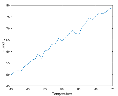
Line plot with x- and y-axis labels that reflect the table variable names

Data Tips: View table variable names as row labels

When plotting tabular data, the default row labels of data tips created interactively or with the datatip function are the names of the table variables associated with the data point.

For example, create a table using the sample file patients.xls. Then, plot the Systolic, Diastolic, and Weight variables in a bubble chart. A data tip created with datatip(b) displays three rows. The row labels are "Systolic", "Diastolic", and "Weight".

tbl = readtable("patients.xls");
b = bubblechart(tbl,"Systolic","Diastolic","Weight");
datatip(b);
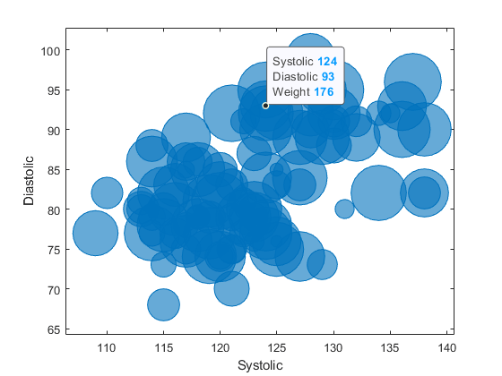
Bubble chart with data tip displaying Systolic 124, Diastolic 93, and Weight 176

Data Tips: View visual property values for scatter plots and bubble charts

For scatter plots and bubble charts, data tips created interactively or with the datatip function include by default rows for visual properties such as size, color, or transparency that are specified with vector data.

For example, create a scatter plot of random data and define the marker sizes as vector sz. A data tip created with datatip(s) displays three rows: X, Y, and Size. The Size row in the data tip displays the marker size specified by sz for the associated data point.

x = linspace(0,3*pi,200);
y = cos(x) + rand(1,200);
sz = linspace(1,100,200);
s = scatter(x,y,sz);
datatip(s);
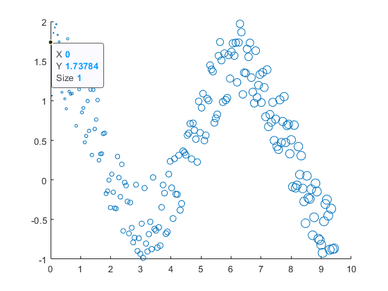
Scatter plot with data tip displaying X 0, Y 1.73784, and Size 1

Bubble Charts and 3-D Scatter Plots: Plot multiple data sets at once

The bubblechart, bubblechart3, polarbubblechart, and scatter3 functions now accept the same combinations of matrices and vectors as the plot function does. As a result, you can visualize multiple data sets at once rather than using the hold function between plotting commands.
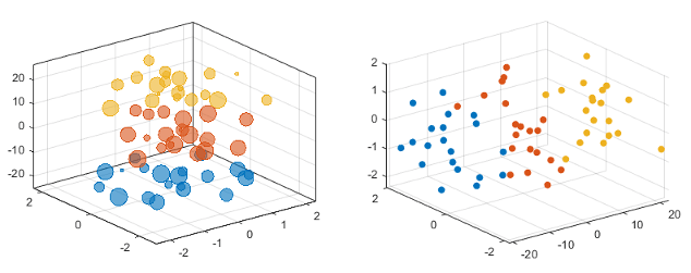
Bubble chart and scatter plot showing multiple data sets. The data sets within each chart have different colors.

fontname and fontsize Functions: Specify the font and font size for graphics objects

Use the fontname and fontsize functions to modify the fonts displayed with graphics objects such as figures, axes, legends, tiled chart layouts, standalone visualizations, and UI components. MATLAB applies your changes to the specified object and all the objects it contains. For example, if you change the font on a figure, all the axes, annotations, and UI components within the figure use the new font.

exportgraphics Function: Create animated GIF files

Create animated GIF files by calling the exportgraphics function multiple times with the Append name-value argument.

Annotation Graphics Objects: Change the annotation rotation angle with the Rotation property

For text box, rectangle, and ellipse annotation objects, rotate the annotation a specified number of degrees by using the Rotation property. The anchor point for rotation is the location specified by the first two elements of the Position property, so the Position property is unaffected by rotation.

For more information, see TextBox Properties, Rectangle Properties, and Ellipse Properties.

Quiver Plots: Align the heads, centers, or tails of arrows with data points

Set the Alignment property of a Quiver object to control how the arrows align with the data points. Valid values are "head", "center", and "tail". For example, plot a grid of vectors with the arrow heads positioned at the data points. Specify a marker symbol to show the locations of the data points.

[X,Y] = meshgrid(0:6,0:6);
U = 0.25*X;
V = 0.5*Y;
quiver(X,Y,U,V,"Alignment","head","Marker","o")
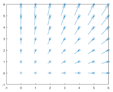
Quiver plot with the arrows pointing at the data points

xlim, ylim, and zlim Functions: Query the axis limit method

Query the method MATLAB uses to set the axis limits by calling the xlim, ylim, and zlim functions and specifying "method" as an input argument.

view Function: Change the view on multiple axes simultaneously

Change the view of multiple axes objects at the same time by passing an array of axes objects to the view function.

rendererinfo Function: Get renderer information without specifying the axes

Call the rendererinfo function without any arguments to query the default graphics renderer information. This new syntax allows you to call the rendererinfo function in a way that is consistent with the opengl syntax. Since R2019a, the rendererinfo function has been recommended instead of the opengl function for querying the renderer.

linkaxes Function: Synchronize axes in all dimensions by default

The linkaxes function now supports 3-D Cartesian axes and synchronizes the x-axis, y-axis, and z-axis limits by default. The supported values of the dimension input argument are now 'xyz' (default), 'x', 'y', 'z', 'xy', 'xz', 'yz', and 'off'.

Before R2022a, linkaxes supported only 2-D Cartesian axes and synchronized the x-axis and y-axis limits by default.

cameratoolbar Function: Syntax support for figures created with the uifigure function

Syntaxes of the cameratoolbar function that do not directly make the toolbar visible are now supported by figures created with the uifigure function.

Callbacks in Live Editor: Create callbacks for figures in the Live Editor

You can now create callbacks for figures created in the Live Editor. The callback workflow supports optional source and event-data parameters.

Keyboard-based callback properties and anonymous function callbacks using Figure objects from the MATLAB workspace are not currently supported in the Live Editor.

To define and execute a figure callback in the Live Editor, use one of these techniques:

  • Create a figure callback and pass source and event data as parameters in the callback.

  • Create a figure callback and do not pass source or event data as a parameter in the callback.

  • Create a callback that includes a function for identifying a graphics object, such as gca or findobj.

For example, define a callback function called colorchangeCallback. With the colorchangeCallback function on the MATLAB path, use the @ operator to assign the function handle to the WindowButtonDownFcn property of the figure fig.

fig = figure;
axis([-4 4 -4 4]);
plot(1:10)
fig.WindowButtonDownFcn = @(src,eventdata)colorchangeCallback(src);

Define the callback and set the Color property for the Axes object in the figure:

function colorchangeCallback(f,~)
% Change the axes color on button down
ax = f.Children;
ax.Color = rand(1,3);
end

For more information, see Callbacks in Live Editor.

Figure Code: Generate code for figure interactions in MATLAB Online

When you modify a figure in MATLAB Online using the Figure tab, MATLAB generates code that you can view, copy, and export. To view the generated code, select Show Code in the File section of the Figure tab. MATLAB generates code for these actions:

  • Adding a title, axis label, legend, color bar, grid, or annotation

  • Changing the text or line style

  • Using the pan, zoom, rotate, or data tip interactions

MATLAB does not currently generate code for the Select and Edit option in the Figure tab.

For example, you can create a surface plot with surf(peaks). Then, interactively add a title and colorbar, zoom into the axes, and view generated code.
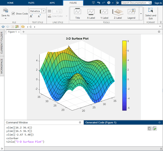
MATLAB Online workspace showing a surface plot with a title and color bar, and generated code. The Show Code check box in the File section of the Figure tab is selected.

 Functionality being removed or changed

Polar axes display angle values with degree symbols

Behavior change

Polar axes now display tick values in degrees with degree symbols when the ThetaAxisUnits property is set to "degrees". For example, create a polar plot. By default, the theta-axis displays the tick values with degree symbols.

theta = 0:0.01:2*pi;
rho = sin(2*theta).*cos(2*theta);
polarplot(theta,rho)
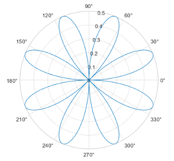
Polar plot that has theta tick values with degree symbols

This change clarifies which units are being used for the theta tick values. You can use the ThetaAxisUnits property to display the tick values in degrees or radians. To remove the degree symbols, change the tick label format for the theta-axis:

pax = gca;
pax.ThetaAxis.TickLabelFormat = "%g";

The caxis function is not recommended

Still runs

The caxis function is no longer recommended. However, the function continues to work, and there are no plans to remove it at this time.

To update your code, call the clim function instead. It accepts the same input arguments and returns the same output as the caxis function.

The im2java function will be removed

Still runs

im2java will be removed in a future release. There is no replacement for this function.

The Plot Catalog tool will be removed

Still runs

The Plot Catalog tool will be removed in a future release. Instead, to interactively create and explore visualizations for your data, use the Plots tab in the MATLAB Toolstrip or the Create Plot task in the Live Editor.

For more information about visualizations, see Types of MATLAB Plots or toolbox-specific documentation.

The opengl function will be removed

Still runs

The opengl function will be removed in a future release.

  • To query the renderer, use the rendererinfo function instead of the opengl function.

  • Changing the renderer with the opengl function will no longer be necessary when the function is removed.

The renderer startup options will be removed

Still runs

In a future release, the MATLAB startup options for selecting the graphics renderer will be removed. Specifically, these startup scenarios will no longer be available:

  • matlab -softwareopengl

  • matlab -nosoftwareopengl

  • matlab -softwareopenglmesa

  • matlab -noopengl

It will no longer be necessary to specify the renderer when these options are removed.

The Renderer property of figures will have no effect

Behavior change in future release

The Renderer and RendererMode properties of figures will have no effect in a future release. It will no longer be necessary to change the renderer when these properties are disabled.

The FontSmoothing property will have no effect

Behavior change in future release

The FontSmoothing property for all types of axes, rulers, geographic scales, and text objects will have no effect in a future release. Font smoothing will be enabled regardless of the value of the property.

Some plot tools functions will redirect to the Figure Toolstrip and Property Inspector

Behavior change in future release

Calling these plot tools functions will open a configuration of the Figure Toolstrip and Property Inspector. For more information, see the Version History section in the documentation for each function.

Currently, calling plot tools functions opens the Figure Palette, Plot Browser, and Property Editor.

App Building

uistyle Function: Add icons and format text in table cells and tree nodes

You can now create styles for table and tree UI components that specify an icon and a text interpreter using the uistyle function.

  • Specify the Icon property of the style object to add icons to table cells and tree nodes.

  • Specify the IconAlignment property of the style object to modify where the icon appears in relation to the text in table cells.

  • Specify the Interpreter property of the style object to format text or add links using HTML markup, or to add equations using TeX or LaTeX markup to table cells and tree nodes.

  • Specify the HorizontalClipping property of the style object to control whether long text is clipped on the left or the right in table cells and tree nodes.

Add a style to a UI component using the addStyle function.

For example, this code creates two styles, one that specifies an icon and one that specifies the text interpreter as TeX, and applies the styles to columns of a table.

T = table(["x^2";"3x^3+1"],["Success";"Success"]);
fig = uifigure(Position=[500 500 300 160]);
t = uitable(fig,Position=[10 10 250 140],Data=T);

s1 = uistyle(Interpreter="tex");
s2 = uistyle(Icon="success",IconAlignment="right");
addStyle(t,s1,column=1)
addStyle(t,s2,column=2)

Table UI component with two columns. The first column contains formatted equations, and the second column contains text with a green check mark icon to the right.

uitable Function: Rearrange columns of table UI components interactively

You can specify the ability to interactively rearrange table columns in an app by using the ColumnRearrangeable property. In a table UI component with the ColumnRearrangeable value set to 'on', rearrange table columns in the app by clicking and dragging the column header.

In App Designer and apps created using the uifigure function, you can program an app to respond when a user rearranges table columns by creating a DisplayDataChangedFcn callback function.

For more information, see Table Properties.

focus Function: Give keyboard focus to UI components programmatically

Use the focus function to programmatically give focus to keyboard-focusable UI components. When a UI component is focused, it is displayed with a blue focus ring, and app users can interact with the component using the keyboard.

isInScrollView Function: Determine if a component is visible in a scrollable container

Use the isInScrollView function to programmatically identify which components are visible given the size and scroll location of a scrollable container. For example, you can determine which axes are visible inside a scrollable figure window and then update the data only for those axes.

 uigridlayout Function: Resize table, list box, and image UI components to fit content

Grid layout managers with row heights or column widths of 'fit' now resize to fit the contents of table, list box, and image UI components.

For example, when you create a table UI component inside a grid layout manager with a row height or column width of 'fit', the height of the row or the width of the column resizes to fit the data in the table.

fig = uifigure(Position=[680 558 300 170]);
gl = uigridlayout(fig);
gl.RowHeight = {'fit'};
gl.ColumnWidth = {'fit'};
tbl = uitable(gl,Data=rand(3));
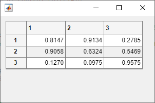
Table UI component. The size of the table is resized to fit the data it contains.

 Compatibility Considerations

In R2021b, grid layout managers with row heights or column widths of 'fit' scaled to a fixed size when the row or column contained a table, list box, or image UI component.

  • Table UI component — Row height and column width previously resized to 300 pixels.

  • List box UI component — Row height previously resized to display at most four items. The exact pixel value to display four items might vary depending on your settings.

  • Image UI component — Row height and column width previously resized to 100 pixels.

To display a table, list box, or image at its size in a release before R2022a, set the corresponding elements of the RowHeight and ColumnWidth properties of the GridLayout object to their respective fixed sizes.

Live Editor Tasks: Develop your own Live Editor tasks for use in live scripts and functions

Live Editor tasks are simple point-and-click interfaces that can be embedded into a live script. Tasks represent a series of MATLAB commands that are automatically generated as users explore parameters.

You can develop your own custom Live Editor tasks by creating a subclass of the LiveTask base class. Develop tasks to perform your own specific set of operations within a live script.

For more information, see Live Editor Task Development Overview.

Custom UI Components: Interactively create custom UI components in App Designer

Use App Designer to interactively build your own UI components. Open a new blank custom UI component in App Designer, lay out the component by combining existing MATLAB UI components or graphics objects, and configure the component interface by creating public properties and public callbacks that can be set when the component is used in an app.

Creating a custom UI component has these benefits:

  • Modularization — Separate the display of large apps into independent, maintainable pieces.

  • Reusability — Provide a convenient interface for adding and customizing similar components in apps.

  • Flexibility — Extend the appearance and behavior of existing UI components.

For more information, see Create a Simple Custom UI Component in App Designer.

App Designer: Modify tab focus order of components

You can view and modify the order in which components in your app receive keyboard focus when the app user presses Tab. First, sort and filter the Component Browser by tab order by selecting Sort & Filter by Tab Order from the drop-down list labeled View. The Component Browser lists only the components in the app that can have focus, in the order of focus. You can then change the tab order of the components by clicking and dragging the component names in the Component Browser.

Alternatively, App Designer can automatically apply a left-to-right and then top-to-bottom tab focus order for components in a container. Right-click the name of the container in the Component Browser and select Apply Auto Tab Order.

App Designer: Specify error handling options and navigate from error messages when debugging an app

To specify error handling options when debugging code in App Designer, configure the Run button by clicking Rundrop-down arrow. You can choose to pause code execution when an error occurs, when a warning occurs, or when a NaN or Inf value is returned.

Additionally, error messages in App Designer now contain links to relevant files and functions. Use these links to navigate more easily to the documentation or to line numbers in your code when debugging your apps.

App Designer: Manage image files in your app with an improved workflow

When you specify image data for your app, such as the image source of an image component or the icon of a button, select an image that is in the same folder as the MLAPP file or one of its subfolders. The image will then load whenever the app is opened or run without it needing to be on the MATLAB path. Alternatively, you can continue to use images in any location by adding the image files to the MATLAB path.

App Designer: Convert components in a grid layout manager to use pixel-based positioning

You can delete a grid layout manager and convert the components in the grid to use pixel-based positioning. To use pixel-based positioning when you were previously using a grid layout manager, right-click the container with the grid layout manager in the canvas, and select Remove Grid Layout.

For more information, see Use Grid Layout Managers in App Designer.

App Designer: Use App Designer in most modern web browsers in MATLAB Online

You can now use App Designer in MATLAB Online with the current versions of Mozilla® Firefox®, Apple Safari, and Microsoft Edge®, in addition to Google Chrome®.

App Designer: Customize design environment layout

You can now customize the locations of the side panels and tabs in the App Designer design environment.

To change the location of side panels such as the Component Library and the Component Browser, click the panel header and drag it to a new location in the App Designer environment. To change the location of your open tabs to display on the left, right, or bottom of the working area, right-click the tab bar and select Tab Position.

Your changes to the design environment layout now persist even after you close and reopen App Designer.

Comparison Tool: Compare and merge app files in MATLAB Online

Compare and merge two versions of an app file in MATLAB Online using the Comparison Tool. To open the Comparison Tool, click Compare in the Designer tab of the App Designer Toolstrip.

For more information, see Compare and Merge Apps.

 Functionality being removed or changed

RearrangeableColumns property of table UI components is not recommended

Still runs

Starting in R2022a, using the RearrangeableColumns property to specify the ability to rearrange columns in a table UI component is not recommended. Use the ColumnRearrangeable property instead. The new property can have the same values as the old one.

There are no plans to remove support for the RearrangeableColumns property at this time. However, the RearrangeableColumns property no longer appears in the list returned by calling the get function on a table UI component.

UIAxes content is not displayed in App Designer Design View when the component is off the canvas

Behavior change

When creating an app with a UIAxes component in App Designer, the UIAxes component content is not displayed in Design View when the component is partially or fully off the canvas. Instead, the UIAxes component is shown as a placeholder image. To see the content of the component, drag it fully onto the canvas.

You can still modify properties of the UIAxes component when it is off the canvas, but you will not be able to see a visual reflection of those changes in Design View until the component is dragged onto the canvas.
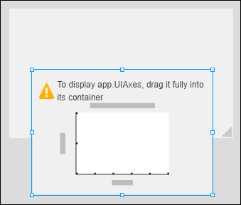
App Designer canvas with a UIAxes component partially off the canvas. The component has a placeholder image with text that says: "To display app.UIAxes, drag it fully into its container".

ComponentContainer class assigns a parent before executing the setup method

Behavior change

When you create an instance of a custom UI component created using the matlab.ui.componentcontainer.ComponentContainer class, the class now assigns the component parent before executing the setup method. As a result, you might see unexpected behavior if your setup method creates underlying UI components that can be parented to either a figure created using the figure function or a figure created the uifigure function, such as panels, tab groups, or button groups.

To update your class code, when you create such a component, specify the property value explicitly for any property where the default value differs depending on the parent. For example, to create a panel in your custom component that is sized using normalized units, specify Units as "normalized" before setting the Position property.

ButtonDownFcn callback cannot be interactively assigned for custom UI components in App Designer

Behavior change

Starting in R2022a, when you use a custom UI component in an app in App Designer, you cannot interactively assign a ButtonDownFcn callback to the component. If you have an existing App Designer app that contains a custom UI component with a ButtonDownFcn callback that you assigned interactively, opening the app in R2022a disconnects the callback from the component. To reassign the callback to the component, follow these steps:

  1. If your app does not contain a StartupFcn callback, right-click the app node from the top of the Component Browser hierarchy and select Callbacks > Add StartupFcn Callback.

  2. In Code View, in the startupFcn function, add this code to assign the appropriate ButtonDownFcn callback programmatically:

    app.CustomUIComponentName.ButtonDownFcn = ...
        @(src,event)CallbackFunctionName(app,event);

    For example, if your app contains a custom UI component named app.IPAddress with a ButtonDownFcn callback named IPAddressButtonDown, add this code to the startupFcn function of your app:

    app.IPAddress.ButtonDownFcn = @(src,event)IPAddressButtonDown(app,event);

Performance

table Data Type Indexing: Improved performance when subscripting with dot notation or multiple levels of indexing

table subscripting when using dot notation is significantly faster in R2022a than in R2021b. Also, subscripting with multiple levels of indexing is faster.

  • For example, when you use dot notation to refer to a table variable with 106 elements, performance in R2022a is more than 4x faster than in R2021b.

    function timingTest()
        t = table(zeros(1e6,1), ones(1e6,1), nan(1e6,1));
        indices = 1:1e5;
        
        tic;
        % Refer to variable using dot notation
        for i = indices
            x = t.Var1;
        end
        toc
    end
    

    The approximate execution times are:

    R2021b: 1.55 s

    R2022a: 0.36 s

  • Similarly, when you use dot notation to assign an array to a table variable with 106 elements, performance in R2022a is about 3x faster than in R2021b.

    function timingTest()
        t = table(zeros(1e6,1), ones(1e6,1), nan(1e6,1));
        indices = 1:1e5;
        x = randi(1e6,1e6,1);
    
        tic;
        % Assign to variable using dot notation
        for i = indices
            t.Var1 = x;
        end
        toc
    end
    

    The approximate execution times are:

    R2021b: 2.15 s

    R2022a: 0.72 s

  • Also, when you use dot notation and parentheses to assign individual values to elements of a table variable, performance in R2022a is more than 4x faster than in R2021b.

    function timingTest()
        t = table(zeros(1e6,1), ones(1e6,1), nan(1e6,1));
        indices = randi(1e6,1,1e5);
    
        tic;
        % Assign to elements using dot notation and parentheses
        for i = indices
            t.Var1(i) = rand;
        end
        toc
    end
    

    The approximate execution times are:

    R2021b: 5.08 s

    R2022a: 1.20 s

The code was timed on a Windows 10, Intel Xeon CPU W-2133 @ 3.60 GHz test system by calling each version of the timingTest function.

Classes: Improved performance for static methods, constant property access, and package functions in scripts

The overhead times for these three actions when performed in scripts are reduced:

  • Executing a package function

  • Executing a static method

  • Accessing a constant property

The overhead times for these actions in a script are now comparable with the times of execution in a function, and the overheads are small enough that they can generally be ignored for performance considerations.

This code performs each of these actions 1,000,000 times. (The code called in each loop is shown at the end of this note.)

tic;
for j = 1:1000000
    out = pkg1.pkg2.packageFunction(2);
end
toc;

tic;
for j = 1:1000000
    out = MyClass.staticMethod(1);
end
toc;

tic;
for j = 1:1000000
    out = pkg1.PackageClass.constantProperty;
end
toc;

The approximate times to complete each loop are:

R2021b:

  • Package function: 8.4 s

  • Static method: 7.8 s

  • Constant property access: 32 s

R2022a:

  • Package function: 0.04 s (210x faster)

  • Static method: 0.031 s (252x faster)

  • Constant property access: 0.039 s (821x faster)

The code was timed on a Windows 10, Intel Xeon CPU W-2133 @ 3.60 GHz test system.

For use with the test code, PackageClass must be in folder +pkg1, and packageFunction must be in folder +pkg1/+pkg2.

function out = packageFunction(in)
    out = in;
end

classdef MyClass
    methods (Static)
        function out = staticMethod(in)
            out = in;
        end
    end
end

classdef PackageClass
    properties (Constant)
        constantProperty = 3;
    end
end

try Block: Improved performance when statements run error-free

The try block shows improved performance when the statements within the block run error-free. For example, this code is approximately 6x faster than in the previous release:

function testTryPerformance
x = 1;
for i = 1:1e8
    try
        x = x * i;
    catch
        warning("Assignment was not successful.")
        x = 1;
    end
end
end

The approximate execution times are:

R2021b: 2.3 s

R2022a: 0.4 s

The code was timed on a Windows 10, Intel Xeon CPU E5-1650 v4 @ 3.60 GHz test system using the timeit function:

timeit(@testTryPerformance)

Python Data Type Conversion: Improved performance when converting between Python and MATLAB data types in out-of-process mode

When you run Python code out of process, conversions between Python data types and MATLAB data types show improved performance.

  • The timingPythonList function converts a Python list object to a MATLAB cell array. This code is about 118x faster than in the previous release:

    function timingPythonList 
        l = py.list(['MATLAB','R',2022,'a','and',1.2,10^2, ... 
            2021,12,25,'2021','12','25','and', ...
            2021,12,25,'2021','12','25']);
        tic
        ml = cell(l);
        toc
    end
    

    The approximate execution times are:

    R2021b: 1.18 s

    R2022a: 0.01 s

  • The timingPythonDict function converts a Python dictionary object to a MATLAB structure. This code is about 57.9x faster than in the previous release:

    function timingPythonDict 
        d = py.dict(pyargs('a',1,'b',2,'c',3,'d',4,'e',5, ...
             'f',6,'g',7,'h',8,'i',9,'j',10,'k',11,'l',12, ...
             'm',13,'n',14,'o',15,'p',16,'q',17,'r',18, ...
             's',19,'t',20));
        tic
        ms = struct(d);
        toc
    end
    

    The approximate execution times are:

    R2021b: 0.521 s

    R2022a: 0.009 s

  • The timingDataTransfer function converts an array with 108 elements from a MATLAB double array to a Python memoryview object and then back to a MATLAB double array. This code is about 10x faster when converting from MATLAB to Python and approximately 11x faster when converting from Python to MATLAB than in the previous release:

    function timingDataTransfer
        data = rand(100,10^6);
        tic
        pydata = py.memoryview(data);
        toc
        tic
        mdata = double(pydata);
        toc
    end
    

    The approximate execution times for converting the MATLAB double array to the Python memoryview object are:

    R2021b: 4.0 s

    R2022a: 0.4 s

    The approximate execution times for converting the Python memoryview object to the MATLAB double array are:

    R2021b: 7.7 s

    R2022a: 0.7 s

All of the code was timed on a Windows 10, Intel Core i7-10510U CPU @ 1.80 GHz 2.30 GHz test system by using Python 3.9 in out-of-process mode and calling the timingPythonList, timingPythonDict, and timingDataTransfer functions.

MATLAB Engine API for Python: Improved performance with large multidimensional arrays in Python

The Python multidimensional array component used by the MATLAB Engine API for Python shows improved performance when:

  1. Converting data from Python sequences to the data types defined by the matlab module

  2. Transferring data back and forth between Python and MATLAB

In both cases, the improvement is noticeable when operating on arrays with at least 10 elements. When transferring data back and forth, the improvement increases as the size of the array increases.

For example, this Python code measures the execution times of two operations:

  1. Converting a Python array of size 108 to a MATLAB double array

  2. Summing the elements of the MATLAB array using the MATLAB engine

The first operation is about 12x faster than in the previous release, and the second operation is about 110x faster than in the previous release:

import random
import time
import matlab.engine
eng = matlab.engine.start_matlab()

rand_array = [random.random() for i in range(10**8)]
s0 = time.perf_counter()
array_md = matlab.double(rand_array,size=(1, 10**8))
s1 = time.perf_counter() - s0
print('conversion to matlab.double(): {} seconds'.format(s1))
s0 = time.perf_counter()
sum_of_elems = eng.sum(array_md,1)
s1 = time.perf_counter() - s0
print('sum(): {} seconds'.format(s1))

The approximate execution times for the first operation are:

R2021b: 42 s

R2022a: 3.6 s

The approximate execution times for the second operation are:

R2021b: 210 s

R2022a: 1.9 s

The code was timed on a Windows 10, Intel Xeon CPU E5-1650 v4 @ 3.60 GHz test system by using Python perf_counter() statements.

Matrix multiplication: Improved performance when multiplying sparse and full matrices

Matrix multiplication shows improved performance when:

  • One of the operands is a sparse matrix, and the other is a full matrix.

  • The sparse operand has at least 50,000 nonzero elements.

  • The full operand has at least 32 columns (or at least 32 rows when transposed).

The performance improvement arises from added support for multithreading in the operation, and therefore the speedup improves as the matrix size and number of nonzero elements increase.

For example, multiplying a 102,400-by-102,400 sparse matrix with a 102,400-by-128 full matrix on a machine with 6 physical cores is about 2.7x faster than in the previous release.

function timingSparseDenseMult
A = delsq(numgrid('S',322));
B = rand(size(A,2),128);
tic
for k = 1:10
    C = A*B;
end
toc
end

The approximate execution times are:

R2021b: 0.8 s

R2022a: 0.3 s

The code was timed on a Windows 10, Intel Xeon CPU W-2133 @ 3.60 GHz test system by calling the timingSparseDenseMult function.

inv Function: Improved performance when inverting large triangular matrices

The inv function shows improved performance when operating on large triangular matrices.

For example, inverting a 5,000-by-5,000 upper triangular matrix is about 3.7x faster than in the previous release.

function timingInv
rng default
A = randn(5e3);
[~,R] = lu(A);

tic
Y = inv(R); 
toc
end

The approximate execution times are:

R2021b: 1.1 s

R2022a: 0.3 s

The code was timed on a Windows 10, Intel Xeon CPU W-2133 @ 3.60 GHz test system by calling the timingInv function.

sprand and sprandn Functions: Improved performance when generating random sparse matrices

The sprand and sprandn functions show improved performance when generating random sparse matrices if the number of nonzero elements in the output is larger than the number of rows.

For example, generating a 10,000-by-10,000 matrix with 10% density of nonzero elements is about 2.5x faster than in the previous release.

function timingSprand
n = 1e4;
d = 0.1; 
rng default

tic
sprand(n,n,d);
toc
end

The approximate execution times are:

R2021b: 2.7 s

R2022a: 1.1 s

The code was timed on a Windows 10, Intel Xeon CPU W-2133 @ 3.60 GHz test system by calling the timingSprand function.

fzero Function: Improved performance

The fzero function shows improved performance for objective functions specified as function handles. This improvement is most noticeable for functions that take little time to evaluate. The following example, which solves for 1e5 roots of a simple function, takes less than one third of the time of the previous release:

N = 1e5;
rng default
levels = 1.5*rand(N,1);
out = zeros(N,1);
tic
for i = 1:N
    out(i) = fzero(@(x)myfun(x,levels(i)),[0 2]);
end
toc

function u = myfun(x,lv)
u = x*sin(x) - lv;
end

The approximate execution times are:

R2021b: 5.83 s

R2022a: 1.66 s

The code was timed on a Windows 10, Intel Xeon CPU E5-1650 v4 @ 3.60 GHz test system by running the above script.

diff Function: Improved performance with large number of elements

The diff function shows improved performance when operating on vectors with at least 105 elements or when operating along the first or second dimension of matrices and multidimensional arrays with at least 5 x 10⁵ elements.

For example, this code creates a double array with 2.5 x 10⁷ elements and calculates differences between adjacent elements. It is approximately 2.4x faster than in the previous release.

function timingDiff
rng default
N = 5000;
A = rand(N);

tic
for k = 1:40
   D = diff(A);
end
toc
end

The approximate execution times are:

R2021b: 2.43 s

R2022a: 1.00 s

The code was timed on a Windows 10, Intel Xeon CPU E5-1650 v4 @ 3.60 GHz test system by calling the timingDiff function.

groupsummary, groupfilter, and grouptransform Functions: Improved performance with small group size

Grouping functions groupsummary, groupfilter, and grouptransform show improved performance, especially when the data count in each group is small.

For example, this code performs group summary computations on a matrix with 500 groups with a count of 10 each. It is about 2.18x faster than in the previous release.

function timingGroupsummary
data = (1:5000)';
groups = repelem(1:length(data)/10,10)';
p = randperm(length(data));
data = data(p);
groups = groups(p);

tic
for k = 1:300
   G = groupsummary(data,groups,"mean");
end
toc
end

The approximate execution times are:

R2021b: 2.14 s

R2022a: 0.98 s

The code was timed on a Windows 10, Intel Xeon CPU E5-1650 v4 @ 3.60 GHz test system by calling the timingGroupsummary function.

nufftn Function: Improved performance with nonuniform sample points or query points

The nufftn function shows improved performance when operating on either nonuniformly spaced sample points or nonuniformly spaced query points.

For example, this code constructs a 32,768-by-3 matrix of nonuniform sample points t and calculates the nonuniform discrete Fourier transform along each dimension of a 32-by-32-by-32 array. The code is about 14.5x faster than in the previous release.

function timingSamplePoints
rng default
t = rand(32^3,3);
X = rand(32,32,32);
tic
  Y = nufftn(X,t);
toc
end

The approximate execution times are:

R2021b: 2.76 s

R2022a: 0.19 s

The code was timed on a Windows 10, Intel Xeon CPU E5-1650 v4 @ 3.60 GHz test system by calling the timingSamplePoints function.

As another example, this code constructs a 65,536-by-3 matrix of nonuniform query points f and calculates the nonuniform discrete Fourier transform along each dimension of a 64-by-32-by-32 array. The code is about 42.6x faster than in the previous release.

function timingQueryPoints
rng default
f = rand(64*32*32,3);
X = rand(64,32,32);
tic
  Y = nufftn(X,[],f);
toc
end

The approximate execution times are:

R2021b: 4.26 s

R2022a: 0.10 s

The code was timed on a Windows 10, Intel Xeon CPU E5-1650 v4 @ 3.60 GHz test system by calling the timingQueryPoints function.

Variables Editor and Live Editor: Improved speed of data display when scrolling

For text and datetime data types in the Variables editor or in the generated output of the Live Editor, the performance of vertical and horizontal scrolling is improved. Displayed data is optimized and the rendering mechanism is faster, so data appears more quickly after scrolling in R2022a than in previous releases.

For example, on a Windows 10, Intel Xeon CPU E5-1650 v4 @ 3.60 GHz test system, when you scroll through a timetable with 3000 rows, the displayed data renders more quickly in R2022a than in R2021b.

App Building: Improved performance when creating UI components

Creating UI components is faster in R2022a than in R2021b. As a result, apps start up faster when you run them. This improvement is more noticeable for apps with many UI components.

For example, this code measures the time it takes to create 500 edit field components. The code is about 1.25x faster than in the previous release.

function timingApp
fig = uifigure;
gl = uigridlayout(fig,Scrollable="on");
gl.RowHeight = repmat({'fit'},1,50);
gl.ColumnWidth = repmat({'fit'},1,10);
drawnow
  
tic
for k = 1:500
    uieditfield(gl);
end
drawnow
toc
end

The approximate execution times are:

R2021b: 7.5 s

R2022a: 6.0 s

The code was timed on a Windows 10, Intel Xeon CPU E5-1650 v4 @ 3.60 GHz test system by calling the timingApp function.

uitable Function and UI Containers: Improved performance when updating properties successively

Updating property values for certain UI components and containers is faster in R2022a than in R2021b. This performance improvement applies to table UI components created using the uitable function, UI containers created using the uipanel, uibuttongroup, uitab, and uitabgroup functions, and custom UI components created using the ComponentContainer base class, when these objects are parented to a figure created using the uifigure function.

For example, this code creates a table UI component and then updates the table cell values for 1000 cells. The code is about 5.2x faster than in the previous release.

function timingTableUpdates
fig = uifigure;
tbl = uitable(fig,"Data",rand(1000,15));
drawnow
 
tic
for k = 1:1000
    tbl.Data(k,1) = 0;
end
drawnow
toc
end

The approximate execution times are:

R2021b: 2.6 s

R2022a: 0.5 s

The code was timed on a Windows 10, Intel Xeon CPU E5-1650 v4 @ 3.60 GHz test system by calling the timingTableUpdates function.

UI Components: Improved performance when setting a property with an unchanged value

Setting a property value of a UI component when the value is unchanged is faster in R2022a than in R2021b. This speed increase leads to improved performance in apps that update many UI component properties at once, even if not all property values have changed.

For example, this code sets the Value property of an edit field to the same value 1000 times. The code is about 23x faster than in the previous release.

function timingValueSet
fig = uifigure;
ef = uieditfield(fig);
drawnow
 
tic
for k = 1:1000
    ef.Value = "Text";
    drawnow
end
toc
end

The approximate execution times are:

R2021b: 2.3 s

R2022a: 0.1 s

The code was timed on a Windows 10, Intel Xeon CPU E5-1650 v4 @ 3.60 GHz test system by calling the timingValueSet function.

App Designer: Improved performance when loading apps with UIAxes components off the canvas

In App Designer, apps with UIAxes components that lie partially or fully off the canvas in Design View have these performance improvements:

  • The app loads faster when you open it.

  • The UIAxes components update faster in response to property edits.

The speed increase improves as the number of UIAxes components that lie off the canvas increases.

For example, create an app in App Designer using these steps:

  1. Drag five UIAxes components onto the canvas.

  2. Drag each of the axes components so that they lie partially off the canvas.

  3. Save and close the app.

Reopen the app. The time it takes for App Designer to fully load the app is about 5.2x faster than in the previous release.

The approximate load times are:

R2021b: 10.5 s

R2022a: 2 s

Once the app is fully loaded, select a UIAxes component and change its title in the Property Inspector. The property updates almost instantaneously. In the previous release, the property update takes approximately 2 seconds.

These interactions were timed on a Windows 10, Intel Xeon CPU E5-1650 v4 @ 3.60 GHz test system.

Plots in Apps: Improved responsiveness for event-driven updates in apps

Apps that involve continuous event-driven updates, such as animations implemented with a timer, are more responsive to those events. To observe the improvement, the animation must be created in an app or in a figure created with the uifigure function. For example, an app containing an animation controlled by a timer object is more responsive when you call the timer’s start and stop methods.

This code creates an app using a timer object to plot a random number every 0.01 second. If you run this app on a Windows 10, Intel Xeon CPU W-2133 @ 3.60 GHz test system, the animation responds more quickly when you click the Start/Stop button than in the previous release.

function mytimerapp
uif = uifigure("CloseRequestFcn",@CloseRequest);
uibutton(uif,"State","Position",[235 59 100 22], ...
    "ValueChangedFcn",@StateButtonChanged,"Text","Start/Stop");
ax = uiaxes(uif,"Position",[25 100 508 300],"XDir","reverse");

% Create initial plot line
p = plot(ax,0:60,zeros(1,61));

% Create timer object
RandTimer = timer(...
    "ExecutionMode","fixedRate", ...
    "Period",0.01, ...
    "BusyMode","queue", ...
    "TimerFcn",@RandTimerFcn);

% Timer function
    function RandTimerFcn(~,~,~)
        % Generate a random number and update plot line
        ydata = p.YData;
        ydata = circshift(ydata,1);
        ydata(1) = rand;
        p.YData = ydata;
    end

% State button callback function
    function StateButtonChanged(obj,~)
        switch obj.Value
            case 0
                stop(RandTimer);
            case 1
                % If timer is not running, start it
                if strcmp(RandTimer.Running,"off")
                    start(RandTimer);
                end
        end
    end

% Figure close request function
    function CloseRequest(~,~)
        % Stop timer, then delete timer and figure
        stop(RandTimer);
        delete(RandTimer);
        delete(uif);
    end
end
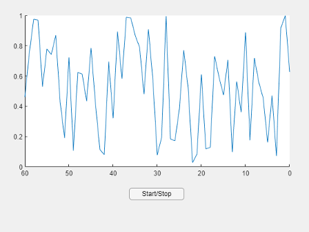
App that plots random numbers every 0.01 second. The app displays the plot and a button for starting and stopping the animation.

Plots in Apps: Improved responsiveness of axes interactions within apps

Responsiveness is improved for panning, rotating, and zooming into a region of interest within a plot. To observe the improvement, the plot must be created in an app or in a figure created with the uifigure function. The improvement is most noticeable for plots with large numbers of points, or those that involve complex effects such as lighting, transparency, or texture maps. Systems equipped with modern GPUs are more likely to show the improvement.

For example, create a 3-D scatter plot with 200,000 points. If you run this code on a Windows 10, Intel Xeon CPU W-2133 @ 3.60 GHz test system with an NVIDIA Quadro P620 GPU, and then drag to rotate the plot, the rotation is smoother and responds more quickly to the drag gesture than in the previous release.

z = linspace(0,4*pi,200000);
x = 2*cos(z) + rand(1,200000);
y = 2*sin(z) + rand(1,200000);
f = uifigure; a = axes(f);
scatter3(a,x,y,z,"filled")
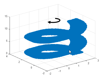
Scatter plot with 200,000 points. A curved arrow is included to represent the rotation interaction.

Plots in Apps: Improved responsiveness of axes interactions in plots with two y-axes

Responsiveness is improved for panning, rotating, and zooming into a region of interest within a UIAxes or Axes object in MATLAB Online that contains a chart created with yyaxis and a legend. For such charts, updates are faster, and interactions are smoother in R2022a than in the previous release.

For example, create a UIAxes object with two y-axes and a legend. If you run this code on a Windows 10, Intel Xeon CPU E5-1650 v4 @ 3.60 GHz test system, when you drag the cursor to pan the view of a UIAxes object, the axes pan faster and track the cursor more closely in R2022a than in R2021b.

f = uifigure;
a = uiaxes(f);
plot(a,1:100,rand(1,100));
yyaxis(a,"right");
plot(a,1:100,linspace(1,10,100));
legend(a);
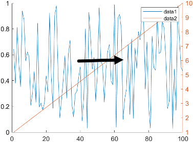
UIAxes object with two y-axes and a legend

Plots in Apps: Faster animations in apps when multiple figures are open

Animations show improved performance in apps when multiple figures are open. To observe the improvement, all figures must be created with the uifigure function.

For example, this code opens 10 empty figures and an additional figure containing a plot. The plot displays one marker that traces the path of a line at every iteration of a loop. The loop is about 6x faster than in the previous release.

function movingmarker

% Open 10 empty figures
for n = 1:10
    uifigure("Position",[10+n*3 10+n*3 200 200]);
end

% Create a figure and a plot with one marker
uif = uifigure;
x = linspace(0,10,200);
y = sin(x);
ax = axes(uif);
p = plot(ax,x,y,"-o","MarkerIndices",1);

% Move the marker along the sine wave
tic
for idx = 2:200
    p.MarkerIndices = idx;
    drawnow
end
toc
end
Plot that displays a marker tracing a sine wave

The approximate execution times for the loop are:

R2021b: 32.6 s

R2022a: 5.4 s

The code was timed on a Windows 10, Intel Xeon CPU W-2133 @ 3.60 GHz test system by calling the movingmarker function.

Property Inspector: Improved performance when opening for the first time

The Property Inspector for a figure window shows improved performance when opening for the first time in a MATLAB session. The delay between clicking the Property Inspector icon or calling inspect and the inspector being ready is reduced. The improvement is most noticeable as the plot in the figure window becomes more complex.

For example, open the Property Inspector for a plot of a 5-by-5 matrix by calling inspect. If you run this code on a Windows 10, Intel Xeon CPU E5-1650 v4 @ 3.60 GHz test system, you can use the Property Inspector sooner in R2022a than in R2021b.

r = rand(5,5);
p = plot(r);
inspect(p)

Software Development Tools

Projects: Reduce test runtime in continuous integration workflows using the dependency cache

You can now specify where your project stores the dependency analysis results. In agile development workflows that use Git and a continuous integration (CI) server, share the dependency cache file (.graphml) to run an incremental dependency analysis and reduce the test suite runtime. See Continuous Integration Using MATLAB Projects and Jenkins.

To set the project dependency cache file, on the Project tab, in the Environment section, click Details. In Dependency cache file, browse to and specify a GraphML file. If the cache file does not exist, the project creates it for you.

Alternatively, you can create and set the project dependency cache programmatically:

matlab.project.example.timesTable
proj = currentProject;
proj.DependencyCacheFile = "myProjectCacheFile"

Dependency Analyzer: Save dependency graph as image

You can now save the dependency analysis results as an image. See Export Dependency Analysis Results.

Code Compatibility Analyzer App: Identify and address compatibility issues against current version of MATLAB

The MATLAB Code Compatibility Report is now available as an app. You can access the Code Compatibility Analyzer from the apps gallery in MATLAB or from the command line using codeCompatibilityAnalyzer. For more information, see MATLAB Code Compatibility Analyzer.

Unit Testing Framework: Create test classes interactively using the Current Folder browser

You can now create a test class using the Current Folder browser in MATLAB and MATLAB Online. To create a new test class, right-click in the Current Folder browser and then select New > Test Class.

Unit Testing Framework: Create temporary folders that are automatically removed

The matlab.unittest.TestCase class has a new method createTemporaryFolder that creates a temporary folder for your tests. The lifecycle of the folder is tied to the test case. Once the test case goes out of scope, the testing framework removes the folder.

Unit Testing Framework: Generate DOCX, HTML, and PDF reports after test execution

The matlab.unittest.TestResult class has three new methods that enable you to generate various test reports from test results. You can run your tests and collect the test results, and then generate test reports from part or all of your results:

With this feature, you are no longer required to run tests using a TestReportPlugin instance. For example, run your tests and then generate an HTML report from the test results. Save the report as report.html in a folder named myResults.

suite = testsuite("MyTestClass");
runner = testrunner;
results = run(runner,suite);
generateHTMLReport(results,"myResults",MainFile="report.html")

Unit Testing Framework: Debug uncaught errors in tests

Starting in R2022a, when a test runner with a StopOnFailuresPlugin instance encounters an uncaught error, MATLAB enters debug mode at the source of the error and lets you use debugging commands to investigate the cause of the error. In previous releases, while the plugin stops the test run to report the error, debugging capabilities are limited because the error disrupts the stack.

Unit Testing Framework: Collect statement and function coverage metrics for your source code

Starting in R2022a, when you generate an HTML code coverage report using the CoverageReport format, the report displays statement and function coverage metrics:

  • Use statement coverage to see whether every MATLAB statement in your source code is executed at least once.

  • Use function coverage to see whether every function in your source code is called at least once.

In previous releases, you can generate only line coverage metrics for your source code. Compared to line coverage, statement and function coverage provide a more detailed analysis of the source code covered by the tests.

 Functionality being removed or changed

pack function will be removed in a future release

Warns

The pack function will be removed in a future release. There is no replacement for this function because you do not need to use it on a 64-bit system. For more information about strategies for reducing memory usage, see Strategies for Efficient Use of Memory and Resolve “Out of Memory” Errors.

matlab.unittest.TestSuite.fromFolder includes tests from package folders when creating a test suite

Behavior change

Starting in R2022a, the matlab.unittest.TestSuite.fromFolder method treats folders and packages the same way, and includes tests defined within package folders when creating a test suite. For example, suite = matlab.unittest.TestSuite.fromFolder(pwd,IncludingSubfolders=true) creates a suite from all the test files in the current folder and any of its subfolders, including package folders. In previous releases, the method ignores any tests defined in a package folder and its subfolders.

This behavior change also applies to the testsuite, runtests, and runperf functions when they operate on a folder containing tests. With the consistent treatment of folders and packages, creating a suite from all test files within a folder and its subfolders becomes more convenient and independent of the folder structure.

To exclude tests defined within packages, filter the suite being constructed or returned by fromFolder. For example, create a filtered test suite comprising tests whose names do not include any dots (that is, do not refer to any packages).

import matlab.unittest.TestSuite
import matlab.unittest.selectors.HasName
import matlab.unittest.constraints.ContainsSubstring
suite = TestSuite.fromFolder(pwd,HasName(~ContainsSubstring(".")), ...
    IncludingSubfolders=true);

builddocsearchdb creates searchable database with new name

Behavior change

When building a searchable documentation database for custom toolboxes, the builddocsearchdb function now creates the subfolder helpsearch-v4 to contain the search database files. Previously, builddocsearchdb created a subfolder named helpsearch-v3.

To ensure the documentation for the custom toolbox is searchable in R2022a, run builddocsearchdb against your help files using MATLAB R2022a. Maintain the helpsearch-v4 subfolder containing the search database files created in R2022a and the helpsearch-v3 subfolder containing the search database files created in previous releases side by side. Then, when you run any MATLAB release, the Help browser automatically uses the appropriate database for searching your documentation.

External Language Interfaces

C++ Interface: Array size help text for functions and methods

If a function or method takes a clib or MATLAB array, the generated help text displays size information for the argument. For more information, see Array Size Help for Functions and Methods.

C Interface: Build third-party C library interface using clibgen.generateLibraryDefinition

Create interfaces for libraries with C files that are built with C compilers using clibgen.generateLibraryDefinition. Use this function to get the benefits of publishing an interface as described in Build MATLAB Interface to C++ Library instead of calling the loadlibrary function described in Call C from MATLAB.

For information about using clibgen.generateLibraryDefinition with C files, see Files in Your Library under the Tips section. To build an interface to C libraries, use the CLinkage name-value argument.

C++ Interface: Support for C++ language features

The C++ interface supports these additional C++ language features.

  • std::complex support for complex scalars and arrays for fundamental types of double, float, int8, uint8, int16, uint16, int32, uint32, int64, and uint64. For information about mapping these types to MATLAB data, see Numeric Types.

  • If the size of a 1-D array parameter is not specified, you can represent the size in MATLAB using multiple dimensions. For example, the input to this function is a 2-D array mat of size len-by-typeSz.

    void readMatrix2DArr(int const [] mat, size_t len, size_t typeSz)
    

    You can specify the SHAPE of the argument as ["len","typeSz"]. For more information, see Define Missing SHAPE Parameter.

  • std::vector as data member.

C++ Interface: Publisher options

The C++ interface supports these build configuration features.

Call MATLAB from C++: Generate C++ code Interface for MATLAB Packages, Classes, and Functions

The matlab.engine.typedinterface.generateCPP creates a C++ header file from MATLAB packages, classes, and functions. For more information, see What is Strongly Typed Interface for C++?.

MATLAB Data Array API: matlab::data::Array support for row-major order

The MATLAB data array API supports iterating through the data of a matlab::data::Array in either row-major or column-major order. For information about specifying the layout when creating an array, see the inputLayout parameter for createArray. For information about iterating through an array, see matlab::data::ColumnMajor, matlab::data::ColumnMajorIterator<T>, matlab::data::RowMajor, and matlab::data::RowMajorIterator<T>.

MEX Functions: UTF-8 system encoding on Windows platforms

MATLAB now uses UTF-8 as its system encoding on Windows, completing the adoption of Unicode across all supported platforms. System calls made from within a MEX file take and return UTF-8 encoded strings. If your MEX file contains code or links to third-party libraries that assume a different system encoding, then you might see garbled text and thus need to update the code to be Unicode compliant.

Python: Use Name=Value syntax to pass keyword arguments to Python functions

You can use MATLAB Name=Value syntax as an alternative to the pyargs function to pass keyword arguments to Python functions. However, do not mix Name=Value arguments with the use of the pyargs function.

MATLAB does not support Name,Value syntax for passing keyword arguments.

Python: Convert Python list and tuple types to MATLAB types

You can convert Python list and tuple types using MATLAB string and numeric converters. For details, see the py.list and py.tuple entry in the Explicitly Convert Python Types to MATLAB Types table. For examples, see Use Python list Variables in MATLAB and Use Python tuple Variables in MATLAB.

Conversion functions might not work on lists or tuples that contain elements which cannot be converted to the requested type:

double(py.list({3.0, 'MATLAB'}))
Error using py.list/double
Conversion of Python element at position 2 to type 'double' failed. All
Python elements must be convertible as scalar to the requested type.

Related documentation

For the related documentation, see Error Converting Elements of list or tuple.

 Perl 5.34.0: MATLAB support on Windows

As of R2022a, MATLAB on Windows ships with an updated version of Perl, version 5.34.0.

 Compatibility Considerations

If you use the perl command on Windows platforms, see https://www.perl.org/ for information about using this version of the Perl programming language.

Compilers: Support for Microsoft Visual Studio 2022

As of R2021b Update 3, MATLAB supports Microsoft Visual Studio 2022 for building C and C++ interfaces, MEX files, and standalone MATLAB engine and MAT-file applications.

 Functionality being removed or changed

Python: Version 3.7 is no longer supported

Errors

Support for Python version 3.7 is discontinued. For continued support for your applications, upgrade to a supported version of Python. For supported version information, see Versions of Python Compatible with MATLAB Products by Release.

MEX file macro FORTRAN_COMPLEX_FUNCTIONS_RETURN_VOID has been removed

Behavior change

For MEX files built in R2021b and earlier, MATLAB provided a macro, FORTRAN_COMPLEX_FUNCTIONS_RETURN_VOID, to handle platform-dependent calling syntax differences for passing complex numbers to Fortran BLAS and LAPACK functions. As of R2022a, you no longer need a different calling syntax on different platforms, and the macro for handling this difference has been removed.

To update your code, replace statements such as these using FORTRAN_COMPLEX_FUNCTIONS_RETURN_VOID:

/* Call BLAS function */
/* Use a different call syntax on different platforms */
#ifdef FORTRAN_COMPLEX_FUNCTIONS_RETURN_VOID
  zdotu(&result, &nElements, zinA, &incx, zinB, &incy);
#else
  result = zdotu(&nElements, zinA, &incx, zinB, &incy);
#endif

with:

/* Call BLAS function */
zdotu(&result, &nElements, zinA, &incx, zinB, &incy);

See dotProductComplex.c.

NET.addAssembly no longer removes leading spaces for Windows drive letter paths

Behavior change

Before R2022a, on Windows platforms, the NET.addAssembly function removed leading spaces in paths specifying the drive letter. If the full path to your assembly is invalid with leading spaces, then remove the spaces before calling NET.addAssembly.

R2021b

New Features, Bug Fixes, Compatibility Considerations

Environment

Editor Selection: Select and edit a rectangular area of code

In the Editor, you now can select a rectangular area in your code (also known as column selection or block edit) by pressing the Alt key while making a selection with the mouse. On macOS systems, use the Option key instead. Selecting and editing a rectangular area of code is useful if you want to copy or delete several columns of data, or if you want to edit multiple lines at one time.

For example, select the second column of data in A.
The variable A, defined as matrix with five columns and three rows. The second column of A is selected.

Type 0 to set all the selected values to 0.
The variable A with the second column in the matrix set to all zeros.

Editor Display: Zoom in and out in the Editor

To zoom in or out in the Editor, go to the View tab, and in the Zoom section, select the Zoom In or Zoom Out button. As you zoom, MATLAB displays the current scale in the bottom-right corner of the Editor. You also can hold the Ctrl key and move the scroll wheel, or press Ctrl+Plus and Ctrl+Minus. On macOS systems, use the Command key and move the scroll wheel, or press Command+Shift+Plus and Command+Shift+Minus.

To return to the default scale, in the View tab Zoom section, select Reset Zoom. You also can press Ctrl+Alt+0 (Command+Alt+0 on macOS).

Editor Code: Show code suggestions and completions automatically

Starting in R2021b, when you write commands in the Editor, MATLAB automatically displays contextual hints for arguments, property values, and alternative syntaxes. In previous releases, MATLAB only completes names in the Editor after a Tab key press.

For example, if you want to use the size function, MATLAB automatically displays the syntax information to help you write the command as you type.
Code suggestion for the size function showing two input arguments, A and dim. The input argument A has the description "input array" underneath it.

MATLAB also automatically suggests and completes the names of functions, models, MATLAB objects, files, folders, variables, structures, graphics properties, parameters, and options.

You can disable automatic completions in the Editor and Live Editor by having MATLAB suggest and complete names only after you press the Tab key. To do so, on the View tab, in the Display section, click the Automatic Completions button off. You also can go to the Home tab, and in the Environment section, click Preferences. Then, select Editor/Debugger > Automatic Completions and in the Suggestions and completions section, select Show on tab.

For more information, see Check Syntax as You Type.

Editor Debugging: Diagnose problems in scripts and functions using inline debugging controls and a breadcrumb-style function call stack

When debugging code in the Editor, you now can diagnose problems using inline debugging controls. For example, to run to a specific line of code and then pause, click the run to here button to the left of the line.

Script with nine lines of code and the run to here button displayed on line two.

To step into a file, click the step in button directly to the left of the function you want to step into. After stepping in, click the step out button at the top of the file to run the rest of the called function, leave the called function, and then pause.

By default, the step in button only appears for user-defined functions and scripts. To show the button for MathWorks functions as well, on the Home tab, in the Environment section, click Preferences. Then, select MATLAB > Editor/Debugger, and in the Debugging in the Live Editor section, clear the Only show Step in button for user-defined functions option.

When you step into a called function or file, the Editor displays an improved breadcrumb-style list of the functions MATLAB executed before pausing at the current line (also called the function call stack). The function call stack is shown at the top of the file and displays the functions in order, starting on the left with the first called script or function, and ending on the right with the current script or function in which MATLAB is paused.

Bread-crumb style function call stack showing the two functions called, displayed left to right. The first function is plotRand the second function is mean. The step out button displays to the right of the function call stack.

For more information, see Debug MATLAB Code Files.

Editor Refactoring: Automatically convert selected code to a function

Break large scripts or functions into smaller pieces by converting selected code into functions in files or local functions. With one or more lines of code selected, on the Editor tab, in the Code section, click the Refactor button, and then select from the available options. MATLAB creates a function with the selected code and replaces the original code with a call to the newly created function.

Editor Code: Automatically complete block endings, match delimiters, and wrap comments while editing code

MATLAB now automatically completes parentheses and quotes when you enter code in the Editor. For example, if you type an open parenthesis in the Editor, MATLAB automatically adds the closing parenthesis. MATLAB also automatically completes comments, character vectors, strings, and parentheses split across two lines.

You also can have MATLAB automatically complete block endings. To do so, on the Home tab, in the Environment section, click Preferences. Select Editor/Debugger > Automatic Completions and in the Autocoding options section, select one or more of the Autocomplete block endings options.

To undo an automatic code completion, press Ctrl+Z or the Undo button. To disable automatic code completions, in the Editor/Debugger > Automatic Completions preferences, clear one or more of the options in the Autocoding options section.

Editor Sections: Create sections with an improved appearance

Starting in R2021b, sections in the Editor have an improved appearance. To create a new section, go to the Editor tab and in the Section section, click the Section Break button. The new section is highlighted with a blue border, indicating that it is selected.
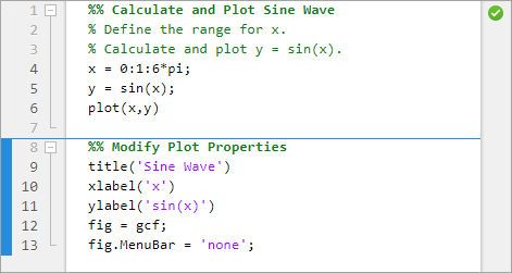
File open in the Editor showing two sections. The second section has a blue border around it indicating that it is the selected section.

To maximize the space available for editing code in the Editor, you can hide the Run to Here and Code Folding margins. This minimizes the gray area to the left of your code. To hide the two margins, right-click the gray area to the left of your code and clear the Show Run to Here Margin and Show Code Folding Margin options.
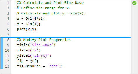
File open in the Editor showing the reduced gray area to the left of the code

As part of this change, the options for changing the appearance of code sections in the Editor have been removed. These options were previously available in the MATLAB > Colors > Programming Tools preferences, in the Section display options section.

For more information about sections in the Editor, see Create and Run Sections in Code.

Editor Code: Change the case of text and code

You can change the case of selected text or code in the Editor from all uppercase to lowercase, or vice versa. To change the case, select the text, right-click, and select Change Case. You also can press Ctrl+Shift+A to change the case. If the text contains both uppercase and lowercase text, MATLAB changes the case to all uppercase.

Editor Bookmarks: Maintain bookmarks after closing a file

Starting in R2021b, MATLAB maintains all bookmarks after you close a file in the Editor. In previous releases, MATLAB does not maintain bookmarks after closing a file.

For more information, see Go To Location in File.

Live Editor Controls: Set default values for sliders, drop-down lists, check boxes, and edit fields

You can set the default values for sliders, drop-down lists, check boxes, and edit fields in your live scripts. To set the default value for a control, right-click the control and select Configure Control. Then, in the Defaults section, specify a default value by entering the value or by selecting a workspace variable from the list. The list shows only valid variables for the control. For drop-down lists, select the default value from the list of items.

To restore the default value for a control, right-click the control and select Restore Default Value.

For more information, see Add Interactive Controls to a Live Script.

Live Editor Animations: Export animations to movies or animated GIFs

Export animations to movies or animated GIFs using the new Export Animation button in the Live Editor animation playback controls. The Export Animation button is not supported for animations generated by the movie function.

For example, this code animates a line growing as it accumulates 2000 data points in the Live Editor. When the animation is done playing, playback controls, including the new Export Animation button, display within the figure window.

h = animatedline;
axis([0 4*pi -1 1])
x = linspace(0,4*pi,2000);

for k = 1:length(x)
    y = sin(x(k));
    addpoints(h,x(k),y);
    drawnow
end
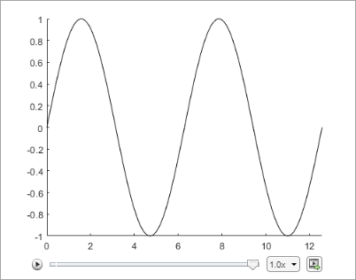
Figure window showing line after animation is done playing. Playback controls, including the new Export Animation button, display below the plot.

For more information about creating animations, see Animation Techniques.

Live Editor Figures: Interact with real MATLAB figures and resize them with improved layouts

Live Editor output figures are now real MATLAB figures with most of the interaction capabilities of standalone MATLAB figures. In addition, when you resize a figure in the Live Editor, the font sizes and spacing between elements in the figure now automatically adjust to provide the best possible presentation for the new size.

Live Editor: Improved performance when saving live scripts or functions

Saving live scripts and live functions in the Live Editor is faster in R2021b than in R2021a. The improvement is most noticeable when you save live functions with more than 1000 lines of code and live scripts with fewer than 100 lines of code.

For example, on a Windows 10, Intel Xeon E5-1650 CPU @ 3.60 GHz test system, saving an example live function containing 4000 lines of code takes approximately 2.05 seconds in R2021b. In R2021a, saving the same live function takes approximately 2.57 seconds.

 Comparison Tool: Compare and merge text files with improved usability, appearance, and syntax highlighting

In R2021b, the comparison tool uses MATLAB Editor syntax highlighting. Text changes and merge choices are now easier to understand. Changes are highlighted with strong colors. Modified lines are highlighted and flagged with the comparison icons , , or . Merging line by line is straightforward, and merge choices are flagged with the merge content icon .

Text comparison report.

 Compatibility Considerations

Starting in R2021b, you no longer can save the comparison report as HTML or specify whether to show only the differences or the entire files.

Importing Preferences from Previous Releases: MATLAB checks for preferences from R2019b or newer

During start up, MATLAB checks for a preferences folder that matches the current release. If that folder is not found, MATLAB checks for preferences folders going back as far as R2019b. Releases before R2021b continue to check for up to three previous releases.

MATLAB ReleasePrevious Release Preferences Folders

R2021b

R2021a, R2020b, R2020a, R2019b

R2021a

R2020b, R2020a, R2019b

R2020b

R2020a, R2019b, R2019a

Display language: MATLAB uses Windows display language settings for selecting desktop language

MATLAB uses the Windows display language settings on Windows 10 to control the MATLAB desktop language. The display language you select on Windows changes the default language used by Windows features like settings and file explorer.

Prior to R2021b, MATLAB controlled the desktop language using the Windows locale setting which is managed in the Region settings.

For information about Windows locale settings in MATLAB, see Set Locale on Microsoft Windows Platforms.

For information about managing display language settings, refer to your Windows 10 documentation.

 Functionality being removed or changed

Increment Value and Run Section tool has been removed

The Increment Value and Run Section tool previously available in the Editor has been removed.

To increment a numeric value within a section, use controls in the Live Editor. For example, this code calculates the factorial of the variable x.

x = 5;
y = factorial(x)
y =
   120
To interactively change the value of x, in a live script, replace the value 5 with a numeric slider. By default, MATLAB reruns the current section when the value of the slider changes.
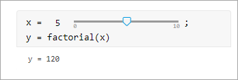
Code that calculates the factorial of x. The value of x is replaced with a numeric slider with a minimum value of 0, a maximum value of 10, and an actual value of 5.

For more information, see Add Interactive Controls to a Live Script.

Language and Programming

cast Function: Consistent output for all syntaxes with the same data type conversion

The cast function now returns consistent output for all syntaxes with the same data type conversion.

For example, starting in R2021b, both b = cast(fi(1),'like',sym(1)) and b = cast(fi(1),'sym') return b = 1 of the sym data type. In previous releases, b = cast(fi(1),'like',sym(1)) returns b = 1 of the sym data type, but b = cast(fi(1),'sym') throws an error.

Run Code in the Background: Use parallel language to run code asynchronously

You can now run code in the background using backgroundPool. When you run code in the background, you can:

  • Run other MATLAB code at the same time as a long running calculation

  • Create more responsive user interfaces

Use the background pool with the following parallel language:

For more information, see Background Processing.

Portable Parallel Code: Share parallel code and seamlessly run in parallel

You can now run parallel code even if you do not have Parallel Computing Toolbox. When you run portable parallel code without Parallel Computing Toolbox, you run the code in serial on your machine. When you run this code with Parallel Computing Toolbox, you can automatically scale up and run the code in parallel on your local machine, on a remote cluster, or in the cloud.

The following parallel language features are available for prototyping:

  • parfeval — Seamlessly run multiple functions at once (since R2021b)

  • parfor — Seamlessly run for-loops in parallel (since R2008a)

For more information, see Run Parallel Language in MATLAB.

Compact Display for Classes: Customize display of information about classes when space is limited

Use the matlab.mixin.CustomCompactDisplayProvider class to customize how information about your classes is displayed in a container variable—such as a struct, cell array, or table—where space is limited. Options for customization include:

  • Displaying partial sets of data

  • Adding annotations

  • Controlling how and when class names are displayed

For example, an enumeration class of the days of the week, WeekDays, can be customized so that when arrays of WeekDays members cannot be fully displayed, MATLAB displays the size, the class, and an annotation. When the width of the Command Window is large enough, the full array is shown:

myStruc = 

  struct with fields:

    prop1: [Monday    Wednesday    Friday    Saturday    Sunday]

When the Command Window is not wide enough to display the full array, the size, the class, and an annotation are shown:

myStruc = 

  struct with fields:

    prop1: 1x5 Weekdays (Enum of days of week)

Class Aliasing: Create aliases for renamed classes to maintain backward compatibility

When you need to change a class name, you can create an alias to preserve compatibility with code written before the name change. The matlab.alias.AliasFileManager class provides an API for defining and implementing aliases. Once you define an alias, you can use the alias anywhere you use the class name. Aliases maintain backward compatibility when reloading objects with the old name into a MATLAB version that uses the new name, as well as forward compatibility when loading objects saved in a newer version into an older version that predates the definition of the alias. MATLAB substitutes the new class name whenever it encounters the old name.

Modular Indexing: Customize class indexing operations individually using new superclasses

To customize how indexing operations behave with your class in previous versions of MATLAB, you need to overload the subsref and subsasgn methods. Doing so requires implementing code for all indexing reference and assignment operations, including parentheses, dot, and brace operations, even if you want to change only one type of indexing operation.

Starting in R2021b, you can inherit from three new superclasses to customize parentheses, dot, and brace indexing operations individually:

You can inherit from one or more of these classes without affecting how the other indexing operations work. These classes also enable you to forward levels of indexing in compound statements to other MATLAB values. For example, your class can implement custom parentheses indexing for the first level of a compound reference and then allow MATLAB to apply the other levels to an object contained by your class.

Scalar Classes: Inherit from the matlab.mixin.Scalar superclass to ensure instances behave as scalars

Instances of classes that inherit from matlab.mixin.Scalar must behave as scalars. You cannot form arrays of instances of such a class, including empty arrays, and you cannot concatenate instances. This class is useful for cases in which concatenation does not make sense, like a dictionary or other container class in which parentheses indexing is customized to access data in the class, not to form or access arrays.

startat Function: Time zone information in datetime objects now supported

The startat function now recognizes time zone and daylight savings time information of datetime inputs.

 Functionality being removed or changed

newclass input argument of the syntax cast(A,newclass) is now case-sensitive

Behavior change

Starting in R2021b, the newclass input argument of the syntax cast(A,newclass) is case-sensitive. You must specify newclass as a character vector or a string of lowercase letters that represents the new data type.

For example, to convert a double value to the int8 data type, you must use b = cast(1.234,'int8'). The function syntax b = cast(1.234,'Int8') now throws an error.

Defining classes and packages: Using schema.m will not be supported in a future release

Still runs

Support for classes and packages defined using schema.m files will be removed in a future release. Replace existing schema-based classes with classes defined using the classdef keyword.

InexactCaseMatch and InexactCaseMatchForExtension Errors: These errors are replaced by UndefinedFunction error

Behavior change

The InexactCaseMatch and InexactCaseMatchForExtension errors have been removed and MATLAB throws an UndefinedFunction error instead. This change does not generate new errors in code that did not previously throw an error.

Data Analysis

Compute by Group Live Editor Task: Interactively summarize, transform, or filter groups of data

Use the Compute by Group Live Editor task to interactively compute statistics, transform data, or filter data by group. To open the task in the Live Editor, use the Task menu on the Live Editor tab.

Normalize Data Live Editor Task: Interactively center and scale data

Use the Normalize Data Live Editor task to visualize the effects of centering and scaling data using various methods, such as the z-score. To open the task in the Live Editor, use the Task menu on the Live Editor tab.

Clean Missing Data Live Editor Task: Define missing values

When using the Clean Missing Data Live Editor task, you can now define missing value indicators that are different from the standard MATLAB missing values.

trenddecomp Function: Find trends in data

Use the trenddecomp function to additively decompose data into a long-term trend and seasonal trends.

min and max Functions: Specify the comparison method for determining minimum and maximum values

The min and max functions now accept the 'ComparisonMethod' parameter, which specifies a method for determining the minimum and maximum values of the input while preserving the sign in the output.

uniquetol Function: Options to control element selection and preserve range of data

uniquetol has two new options to control behavior:

  • occurrence argument: Specify whether the algorithm begins with the highest or lowest elements in the input data. This can change which element, among several that are within tolerance of each other, is selected as being unique. The default is to begin with the lowest elements.

  • 'PreserveRange' name-value argument: Specify whether the range of the output data should be the same as the input data.

Data Preprocessing Functions: Specify table variable as sample points vector

When you operate on table input data, the following functions now allow you to specify which variable in the table to use with the 'SamplePoints' parameter:

dateshift Function: Shift to next occurrence of weekday or weekend day

You can now use the 'weekday' and 'weekend' arguments to shift the elements of a datetime array when using the dateshift function.

  • To shift to the next occurrence of a weekday on or after each element of the input datetime array, use 'weekday'.

  • To shift to the next occurrence of a weekend day on or after each element of the input datetime array, use 'weekend'.

isbetween Function: Support for open, closed, and half open intervals

The isbetween function now supports open, closed, and half open intervals. In previous releases, isbetween supports only closed intervals.

isregular Function: Support for datetime and duration data types

You can now use the isregular function to determine if a timetable, datetime vector, or duration vector is regular. In previous releases, you can use isregular only on a timetable.

istabular Function: Determine if input is a table or timetable

To determine if an input variable is either a table or a timetable, use the istabular function.

Using this function is equivalent to using the statement tf = istable(A) || istimetable(A), but is more convenient.

retime and synchronize Functions: Median and mode methods supported

When you synchronize data in timetables, you can now specify 'median' and 'mode' as aggregation functions. For more information, see retime and synchronize.

timeofday Function: Return the date as the second output argument

You can now return the dates from the elements of a datetime array as the second output argument from the timeofday function.

timeseries2timetable Function: Convert timeseries objects to timetables

To convert timeseries objects to timetables, use the timeseries2timetable function.

 Functionality being removed or changed

isordinal accepts input argument that has any data type

Behavior change

The isordinal function now accepts an input argument that has any data type. In previous releases, isordinal threw an error if the input argument was not a categorical array.

Synchronize Timetables Live Editor task synchronizes an unlimited number of timetables

Behavior change

The Synchronize Timetables Live Editor task can now synchronize an unlimited number of timetables. In previous releases, the task can synchronize no more than five timetables.

timeseries2timetable replaces ts2timetable

Behavior change

The timeseries2timetable function replaces the ts2timetable function, although ts2timetable is still provided. The two functions are synonyms. In R2021a, MATLAB provides ts2timetable only.

Data Import and Export

sftp Function: Connect to SFTP servers

MATLAB can connect to SFTP servers for encrypted data transfers. Create an SFTP connection object using the sftp function to read data from an SFTP server.

Datastores: Specify FileSet objects as data locations for some datastores

Some datastore functions and objects accept FileSet objects as the locations of files to include in the datastore. FileSet objects provide increased performance compared to file paths or DsFileSet objects. This functionality is supported by these functions:

  • tabularTextDatastore

  • spreadsheetDatastore

  • fileDatastore

  • keyValueDatastore

  • tallDatastore

  • parquetDatastore

  • imageDatastore

  • signalDatastore (Signal Processing Toolbox)

  • audioDatastore (Audio Toolbox)

  • mdfDatastore (Vehicle Network Toolbox)

Table Import: Read tables from HTML and Microsoft Word documents

The readtable function now supports reading tables from HTML and Microsoft Word files.

To customize import options for HTML and Microsoft Word files, use htmlImportOptions and wordDocumentImportOptions, respectively. To automatically detect import options from files, use the detectImportOptions function.

HDF5 Interface: Use new functionality in support of HDF5 1.10.7

Use these new capabilities of the MATLAB HDF5 function interfaces:

  • Single-Writer/Multiple-Reader (SWMR) — Write data to an HDF5 file in one process while you concurrently read from the file in one or more reader processes. For more information, see Read and Write Data Concurrently Using Single-Writer/Multiple-Reader (SWMR).

  • Virtual Dataset (VDS) — Use the MATLAB low-level interface to access data stored across multiple HDF5 files, including files in remote locations, as a single, unified HDF5 dataset. You can also read data stored in Virtual Datasets using the HDF5 high-level interface. For more information, see Work with HDF5 Virtual Datasets (VDS).

  • Metadata Cache Fine-Tuning — Improve performance by controlling the parameters of the metadata cache, such as limiting the number of file reading attempts.

  • Partial Edge Chunk — Control whether to filter partial edge chunks.

NetCDF Interface: Read and write NC_STRING data

You can now use the existing high-level and low-level functions to read NC_STRING data from NetCDF-4 files and write text data as type NC_STRING.

For more information on data type mapping between the NetCDF API and MATLAB, see Map NetCDF API Syntax to MATLAB Syntax.

Scientific File Format Libraries: HDF5 and NetCDF libraries are upgraded

The HDF5 library is upgraded to version 1.10.7, and the NetCDF library is upgraded to version 4.7.4.

Audio, Video, and Image I/O Functions: Run functions in a thread-based environment

You can now run the following functions in the background using MATLAB backgroundPool:

For more information, see Run MATLAB Functions in Thread-Based Environment.

Image File Format Libraries: LibTIFF library upgraded to version 4.2.0

The LibTIFF library is upgraded to version 4.2.0.

New Serial Explorer and TCP/IP Explorer apps

Two new apps offer functionality for communicating with your device, instrument, or server:

  • The Serial Explorer app provides a user interface to connect to and communicate with a serial port device on your machine.

  • The TCP/IP Explorer app provides a user interface to create a TCP/IP client that communicates with a TCP/IP server.

Launch these apps from the Apps tab, under the Test and Measurement section. You can also call the serialExplorer and tcpipExplorer commands in the Command Window.

You can use the apps to perform the following operations on your serial port device or TCP/IP client.

  • Configure connection and communication properties.

  • Write binary or string data.

  • Read binary or string data.

  • Plot data in a separate figure window.

  • Analyze data by viewing it in the Signal Analyzer app.

  • Export data to the MATLAB workspace.

  • Generate a MATLAB script for app interactions that uses the serialport or tcpclient interface.

For more information about these apps, see Serial Explorer and TCP/IP Explorer.

 Functionality being removed or changed

Video and Image I/O Functions: Pixel value differences might exist between JPEG 2000 images in R2021b and previous versions of MATLAB

Behavior change

In R2021b, when you use the imread, imwrite, VideoReader, or VideoWriter functions to read or write JPEG 2000 image files, the image you import or export in R2021b might have pixel value differences with the same image in previous versions of MATLAB.

HDF5 Interface: Linux users need to rebuild filter plugins using MATLAB HDF5 1.10.7 shared library

Behavior change

Starting in R2021b, in certain cases, Linux users using a filter plugin with callbacks to core HDF5 library functions need to rebuild the plugin using the shipping MATLAB HDF5 1.10.7 shared library, /matlab/bin/glnxa64/libhdf5.so.103.3.0. If you do not rebuild the plugin using this version of the shared library, you might experience issues ranging from undefined behavior to crashes. For more information, see Build HDF5 Filter Plugins on Linux Using MATLAB HDF5 Shared Library or GNU Export Map.

ftp Function: FTPClientConfig class, properties, and methods are no longer supported

The ftp function no longer supports the Apache® FTPClientConfig class or any associated objects, properties, or methods. To customize how to parse the LIST command output of the FTP server use the ftp function’s DirParserFcn name-value argument.

MATLAB Variable Editor: timeseries will no longer be supported in a future release

Still runs

Viewing timeseries objects using the MATLAB Variable Editor will no longer be supported in a future release. To view time-indexed data in the Variable Editor, use timetable instead.

Mathematics

ode78 and ode89 Functions: High-order Runge-Kutta solvers for ordinary differential equations

The MATLAB ODE suite has been expanded with two new solvers:

  • ode78 uses 7th- and 8th-order Runge-Kutta formulas

  • ode89 uses 8th- and 9th-order Runge-Kutta formulas

The new solvers expand on the existing Runge-Kutta solvers ode23 and ode45. In particular, ode78 and ode89 can be more efficient than ode45 on nonstiff problems that are smooth, and ode89 can be more efficient than ode78 on very smooth problems, when you integrate over long time intervals or when tolerances are tight.

pagesvd Function: Perform singular value decomposition on pages of N-D arrays

Use the pagesvd function to perform batched singular value decompositions on the pages of N-D arrays. In this context, the N-D array is treated as a container for several 2-D matrices.

svd Function: Option to control output format of singular values

svd has a new option outputFormat to control whether the singular values are returned as a vector or diagonal matrix.

mpower Function: Improved algorithm for defective matrices

The mpower function has an improved algorithm to handle defective matrices raised to a real power. In previous releases, mpower uses an algorithm based on eigenvalue decomposition for these inputs that can return incorrect results for defective matrices. The new algorithm for defective matrices is instead based on the Schur decomposition.

 Functionality being removed or changed

svd, eig, cond, and pinv functions return NaN for nonfinite inputs

Behavior change

In R2021b, the svd, eig, cond, and pinv functions return NaN values when the input contains nonfinite values (Inf or NaN).

In previous releases, these functions throw an error when the input contains nonfinite values.

Graphics

Plotting Table Data: Create scatter plots, bubble charts, and swarm charts by passing tables directly to plotting functions

Create plots by passing a table directly to any of these functions: scatter, scatter3, bubblechart, bubblechart3, swarmchart, swarmchart3, polarscatter, and polarbubblechart. When you specify your data as a table, the axis labels and the legend (if present) are automatically labeled using the table variable names.

The objects returned by these functions have new properties to support tables.

PropertyDescription

SourceTable

Table containing the data to plot

XVariable, YVariable, and ZVariable

Table variables containing the x, y, and z values for Cartesian plots

ThetaVariable and RVariable

Table variables containing the angle and radius values for polar plots

SizeVariable

Table variable containing the marker size data

ColorVariable

Table variable containing the marker color data

AlphaVariable

Table variable containing the marker transparency data

For example, create a table with the variables "Trials" and "Response". Pass the table to the scatter function as the first argument, and indicate the variables you want to plot by name.

Trials = randi(10,50,1);
Response = rand(50,1);
t = table(Trials,Response);
scatter(t,"Trials","Response")
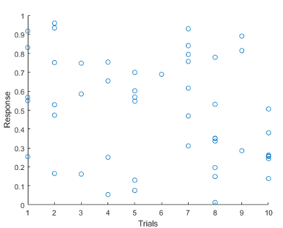
Scatter plot with x- and y-axis labels that reflect the table variable names.

Axes Ticks and Colors: Control the appearance of axis tick marks and tick label colors

Now, you can remove tick marks and customize tick label colors independently of other elements in the axes.

  • Removing Tick Marks — Remove all the tick marks from an axes, polar axes, or geographic axes object by setting the TickDir property to 'none'. To remove the tick marks from a specific axis, for example the x-axis, set the TickDirection property of the ruler to 'none'.

  • Customizing Tick Label Colors — Customize the color of the tick labels on an axis by setting the TickLabelColor property of the corresponding ruler object. You can customize tick label colors for any axes, polar axes, or geographic axes.

For example, create a bar chart, and then get the current axes. Remove the x-axis tick marks and change the color of the x-axis tick labels to red.

bar([2017 2018 2019 2020],1:4)
ax = gca;
ax.XAxis.TickDirection = 'none';
ax.XAxis.TickLabelColor = 'r';
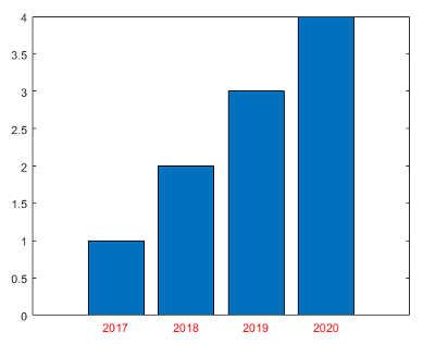
Scatter plot with x-axis label and legend labels that reflect the table variable names.

Create Plot Live Task: Add additional visualizations to generated plots

Easily add additional visualizations to plots generated using the Create Plot Live Task. To add a new plot, click the Add tab at the bottom of the Live Task Panel and select the visualization and data. This Live Task combines the plot using the hold function.
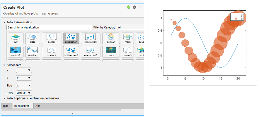
A Screen shot of the Create Plot Live Task showing a line plot of a sine wave in blue and a bubble plot of a cosine wave in orange.

Create Plot Live Task: Control chart input syntax using configuration drop-down

The Create Plot Live Task now supports multiple configurations of charting functions with multiple input syntaxes, including surf and mesh. Use the Configurations drop-down menu to select the desired configuration.
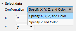
A screenshot of the configuration drop-down menu for a surf plot

exportgraphics Function: Capture and append graphics to existing PDFs

Capture and append graphics to an existing PDF file by calling the exportgraphics function and setting the 'Append' name-value argument to true. For example, create a plot and export it as a PDF called 'mycharts.pdf'. Then, create a bar chart and append it to the end of 'mycharts.pdf'. The resulting PDF file has two pages. The plots appear in the PDF in the order that you export them.

plot([0 3 1 6 4 10])
exportgraphics(gca,'mycharts.pdf')
bar([10 20 30 40])
exportgraphics(gca,'mycharts.pdf','Append',true)

stackedplot Function: Support for semilog y-axes

You can create plots using the stackedplot function where individual y-axes can be plotted on a log scale. To set a log scale for the y-axis of a plot, set the YScale property of the StackedAxesProperties object associated with the plot. For more information, see StackedAxesProperties Properties.

Text Objects: Use editInteractions in the Interactions property to click or tap on text to edit

Click or tap to edit text when the Interactions property has the value editInteraction. The edit interaction is default behavior for title, subtitle, xlabel, ylabel, and zlabel text objects for axes, geographic axes, and polar axes.

dataTipTextRow Function: Customize data tip content using data properties, such as UserData

You can now assign information to the DataTipTemplate property by passing it to the dataTipTextRow function as a property name, such as UserData.

p = patch;
p.UserData = p.XData;
p.DataTipTemplate.DataTipRows(3) = dataTipTextRow('XDataAsUserData','UserData');

MATLAB Online™ Accessibility: Use a screen reader to interact with figures

In MATLAB Online™, you can use a screen reader and keyboard commands to pan, zoom, and rotate when you work with plotted data. Using a screen reader is not supported in the Live Editor.

For more information, see Use a Screen Reader in MATLAB Online.

For more details on interacting with MATLAB figures, see Control Chart Interactivity.

 Functionality being removed or changed

The print options -opengl and -painters are not recommended

Still runs

The following print options are no longer recommended. There are no plans to remove the values, and they will continue to behave the same way as in previous releases. The following table lists the recommended replacement options.

Not RecommendedReplacement Option

The -opengl renderer option. For example:

print('-opengl','-dpdf','myfigure.pdf')

Use the -image option. For example:

print('-image','-dpdf','myfigure.pdf')

The -painters renderer option. For example:

print('-painters','-dpdf','myfigure.pdf')

Use the -vector option. For example:

print('-vector','-dpdf','myfigure.pdf')

plottools functions will be removed in a future release

Still runs

The plottools functions listed below will be removed in a future release. Use inspect to launch the Property Inspector instead.

plottools functions

App Building

uialert, uiconfirm, and uiprogressdlg Functions: Mark up text and display equations in dialog boxes

When you create dialog boxes using the uialert, uiconfirm, and uiprogressdlg functions, enable markup in the dialog box text using the Interpreter name-value argument. Specify the interpreter as 'html', 'latex', 'tex', or 'none'.

addStyle Function: Add styles to nodes and levels in a tree UI component

Create styles for specific tree nodes or tree node levels in a tree UI component using the uistyle and addStyle functions. For example, you can make the tree nodes at the top level of the tree red with italic font. To get information on applied styles, query the StyleConfigurations property of the Tree object. To remove a style from a tree, use the removeStyle function.

uitable Function: Set and query table selections programmatically and control table selection options

You can now configure selection options of table UI components.

  • Set and query the table selection using the Selection property.

  • Specify whether a user can select table cells, rows, or columns using the SelectionType property.

  • Specify whether a user can select single or multiple table elements using the Multiselect property.

  • Update your app whenever a user selects table data by specifying a SelectionChangedFcn callback.

Selection options in table UI components are supported only in App Designer apps and in figures created with the uifigure function.

For more information, see Table Properties.

uitextarea Function: Program apps to respond while a user is typing in a text area component

You can now specify a ValueChangingFcn callback for a TextArea component. The component executes the callback function repeatedly while a user types in the text area.

For more information, see TextArea Properties.

Run Code in the Background: Use parallel language to create more responsive apps

You can now create apps that remain responsive while performing calculations in the background by using backgroundPool.

Use the background pool with the following parallel language:

For more information, see Use the Background to Make Your Apps More Responsive.

App Designer: Debug code in Code View

When debugging code in App Designer, you now can diagnose problems using debugging controls in Code View. You can use the controls in the Run section of the Editor tab to run to the next breakpoint, run the next line of code, or step into or out of a function.
Debugging controls in App Designer. There are five buttons: Continue, Step, Step In, Step Out, and Stop.

You can also debug your app code using inline debugging controls. For example, to run to a specific line of code and then pause, click the run to here button to the left of the line. To step into a function, click the step in button directly to the left of the function you want to step into. After stepping in, click the step out button at the top of the file to run the rest of the called function, leave the called function, and then pause.

When you step into a called function or file, App Designer displays a breadcrumb-style list of the functions MATLAB executed before pausing at the current line (also called the function call stack). The function call stack is shown at the top of the file and displays the functions in order, starting on the left with the first called script or function, and ending on the right with the current script or function in which MATLAB is paused.

Bread-crumb style function call stack showing the two functions called, displayed left to right. The first function is plotRand the second function is mean. The step out button displays to the right of the function call stack.

 App Designer: Efficiently manage your app code with tools and shortcuts from Live Editor

Many of the tools and shortcuts for navigating and organizing code that are available in the Live Editor can now be used in App Designer Code View. This table lists the functionality that is new to App Designer.

FunctionalityMenu ItemKeyboard Shortcut
Wrap comment

Right-click the comment and select Wrap Comments, or in the Editor tab, in the Code section, click the Wrap comment button.

Ctrl+J
Navigate code using bookmarks

In the Editor tab, in the Navigate section, click Bookmark. Then, select Bookmark to set or clear a bookmark on the current line, or select Previous or Next to navigate between the existing bookmarks.

Drop-down with bookmark options

Set or clear bookmark: Ctrl+F2
Move to previous bookmark: Shift+F2
Move to next bookmark F2
Print app code

In the Editor tab, in the File section, click Print. You can print the entire document or the current selection.

App designer print options menu.

Ctrl+P
Fold and expand code

In the View tab, click the buttons in the Code Folding section.

Code folding options to expand, collapse, expand all, or collapse all.

Expand current fold: Ctrl+Shift+Period (.)
Collapse current fold: Ctrl+Period (.)
Expand all folds: Ctrl+Shift+Comma (,)
Collapse all folds: Ctrl+Comma (,)
Toggle display preferences

In the View tab, in the Display section, toggle line highlighting and line numbers.

App Designer display options. The options are: Highlight Current Line, Line Numbers, and Datatips.

N/A
Duplicate lineRight-click a line and select Duplicate Line(s). Ctrl+Shift+C
Insert section breakRight-click a line and select Section Break.Ctrl+Alt+Enter, or type %%
Convert text to uppercase or lowercaseHighlight the text, right-click it, and select Change Case.Ctrl+Shift+A
Variable rename

When you rename a variable, App Designer gives you the option to automatically update all other instances of the variable in your code.

Tooltip prompting variable renaming in App Designer

Shift+Enter
 Compatibility Considerations

Code folding in App Designer persists even after you close and then reopen the file. In R2021a and earlier releases, when opening a file, App Designer expands all the code.

App Designer: Interactively modify canvas zoom level and fit canvas to view

In Design View, use the zoom controls in the lower right corner of the App Designer canvas, indicated by the Zoom icon button, to modify the canvas zoom level.

To automatically zoom to fit the entire app in the view, press Space. Alternatively, click Fit to View in the Zoom section of the View tab, or right-click on the canvas and select Zoom > Fit to View.

App Designer: Convert between similar UI components

To convert one type of UI component to another with similar functionality, right-click the component on the canvas or in the Component Browser and select Replace With. Then, select the component to convert to. Replacing one component with another preserves relevant property values, such as font properties and callbacks that exist for both components. You can convert component types within each of these families:

  • Numeric edit field, spinner, slider, and knob

  • Edit field and text area

  • Label and hyperlink

App Designer: Add help text for your app

You can now provide help for apps that you create. Help text appears in the Command Window when an app user calls the help function and specifies the name of the app.

To add help text, in the Editor tab in Code View, click App Help Text. Use the App Help Text dialog box to specify the app summary and detailed explanation.

In addition, when an app user views the documentation for your app (for example, by calling the doc function or by clicking the documentation link in the help text for the app), the documentation page now displays additional information:

  • The top of the page displays the app summary and detailed explanation.

  • The Methods Summary section displays the public functions. For each function, it also displays any comment that is inserted after the function definition statement.

App Designer: Remove auto-reflow behavior from an app with auto-reflow

To convert an app with auto-reflow to an app without auto-reflow, in the Canvas tab in Design View, click Convert. Select the App without Auto-Reflow option. Doing so creates a duplicate of your app with the auto-reflow behavior removed.

For more information, see Apps with Auto-Reflow.

Deployed Web Apps: Deploy web apps directly to the MATLAB Web App Server from within App Designer

Once you have MATLAB Compiler™ installed on the system running MATLAB, package your MATLAB app into a web app from within App Designer by clicking Share in the Designer tab and selecting Web App. In the packaging dialog, specify the server URL to directly deploy your web app to the server once packaging is complete. Authentication must be enabled on the server for this to work. For details, see Authentication (MATLAB Web App Server).

App Testing Framework: Perform press gestures on axes and UI axes with different selection types

The app testing framework now supports mouse selection types in press gestures that are performed on axes and UI axes. For example, create an axes with a plot and then test a double-click gesture at the point (3, 2).

f = uifigure;
ax = axes(f);
plot(ax,1:10)
tc = matlab.uitest.TestCase.forInteractiveUse;
tc.press(ax,[3 2],'SelectionType','open')

App Testing Framework: Perform drag gestures on axes and figures with different selection types

Starting in R2021b, the app testing framework supports drag gestures on UI figures. Additionally, when you test a drag gesture on an axes, UI axes, or UI figure, you can specify the mouse selection type. For example, create a figure and drag on it from the point (100, 200) to the point (200, 300) using a right-click gesture.

f = uifigure;
tc = matlab.uitest.TestCase.forInteractiveUse;
tc.drag(f,[100 200],[200 300],'SelectionType','alt')

App Testing Framework: Use any units of measurement in gestures at the center of components

Starting in R2021b, when you perform a gesture at the center of a component, the component or its parent containers can use any units of measurement. In previous releases, the framework does not support containers that use nonpixel units.

For example, create a figure and set its Units property to 'normalized'. Then, create a panel in the figure and press at the center of the panel.

f = uifigure;
f.Units = 'normalized';
p = uipanel(f);
tc = matlab.uitest.TestCase.forInteractiveUse;
tc.press(p)

If you perform a gesture at the center of a component using a syntax that accepts location as an input (for instance, press(testcase,comp,location)), then the figure or parent containers can use only 'pixels' as their units of measurement.

 Functionality being removed or changed

Ctrl+Click selects and deselects cells in a table UI component

Behavior change

In tables created using the uitable function, you can select and deselect noncontiguous table cells by holding Ctrl and clicking a cell. In R2021a and earlier releases, Ctrl+Click gives focus to a cell and Shift+Click selects the cell that has focus.

App Designer toolstrip organization has changed

Behavior change

The organization of the tools in the App Designer toolstrip in Design View and Code View has changed.

In Design View, use the tools in the Canvas tab to lay out your app, and use the tools in the View tab to manage your Design View preferences.

In Code View, use the tools in the Editor tab to program your app behavior and to run and debug your app, and use the tools in the View tab to manage your Code View preferences.

matlab.fonts.editor.codefont.Size setting has been removed

Errors

The matlab.fonts.editor.codefont.Size setting has been removed. Use the matlab.fonts.codefont.Size setting instead. The matlab.fonts.codefont.Size setting controls both the App Designer Code View font size and the desktop code font size.

To update your code, change instances of the setting matlab.fonts.editor.codefont.Size to matlab.fonts.codefont.Size. For more information, see matlab.fonts Settings.

App Designer Smart Indent applies to individual lines

Behavior change

When you apply Smart Indent to code in App Designer, the indentation change applies only to the current line. In R2021a and earlier releases, the Smart Indent option applied to the entire document.

To apply Smart Indent to the entire document, in Code View, first select all the code (for example, by pressing Ctrl+A). Then, apply Smart Indent by clicking the Smart indent button in the Editor tab, or pressing Ctrl+I.

CellSelectionCallback property of table UI components is not recommended in uifigure-based apps

Still runs

Starting in R2021b, using the CellSelectionCallback property to program a response to table selection is not recommended for table UI components in App Designer apps and in figures created with the uifigure function. Use the SelectionChangedFcn property instead.

To update your code, assign all callback functions assigned to the CellSelectionCallback property to the SelectionChangedFcn property instead. If a callback function accesses the callback event data, you might need to update the event property names. For example, to access the indices of the elements the user selected, use the Selection property of the TableSelectionChangedData object. For more information, see Table Properties.

Performance

table Data Type Indexing: Improved performance when assigning elements by subscripting with curly braces

table subscripted assignment using curly braces is significantly faster in R2021b than in R2021a.

For example, when you assign into three table variables with 106 elements, performance in R2021b is approximately 4.4x faster, as shown below.

function timingTest()
    t = table(zeros(1e6,1), ones(1e6,1), nan(1e6,1));
    indices = randi(1e6,1,10000);

    tic;
    % Assign row vector of random values to randomly chosen row
    for i = indices
        t{i,:} = rand(1,3);
    end
    toc
end

The approximate execution times are:

R2021a: 7.4 s

R2021b: 1.7 s

The code was timed on a Windows 10 system with a 3.6 GHz Intel Xeon W-2133 CPU by calling the timingTest function in R2021a and R2021b.

qrinsert and qrdelete Functions: Improved performance modifying QR factorizations

The qrinsert and qrdelete functions show improved performance inserting and deleting rows and columns in a QR factorization. The speedup is most noticeable for square matrices of order 1000 or less and is similar in magnitude for both rows and columns.

For example, this code uses a loop to insert and delete columns from the QR factorization of a random 200-by-200 matrix. qrinsert and qrdelete are about 12x faster than in the previous release.

function timingQRMod
X = rand(200);
[Q,R] = qr(X);
y = rand(200,1);
tic
for k = 1:1000
    [Qn,Rn] = qrinsert(Q,R,100,y);
end
toc
tic
for k = 1:1000
    [Qn,Rn] = qrdelete(Q,R,100);
end
toc
end

The approximate execution times are:

R2021a: 1.7 s (insertion) and 1.2 s (deletion)

R2021b: 0.15 s (insertion) and 0.10 s (deletion)

The code was timed on a Windows 10, Intel Xeon W-2133 CPU @ 3.60 GHz test system by calling the timingQRMod function.

Titles and Labels in Plots: Improved performance when creating and querying titles or labels in a loop

Creating and querying the following types of titles and labels in a loop has improved performance.

  • Plot titles, such as those created with the title or subtitle functions

  • Axis labels, such as those created with the xlabel, ylabel, or zlabel functions

For example, this code creates 100 axes with titles in a tiled chart layout. It runs 11.9x faster than in the previous release:

function timingTitle
tiledlayout(10,10);
for n = 1:100
    nexttile
    title(n)
end
end

The approximate execution times are:

R2021a: 9.5 s

R2021b: 0.8 s

The code was timed on a Windows 10, Intel Xeon CPU E5-1650 v4 @ 3.60 GHz test system by calling the timeit function:

timeit(@timingTitle)

The performance gains increase with the number of axes, titles, and axis labels you are working with. For example, this table shows the improvements for looping over 10, 20, 50, and 100 axes with titles.

Number of Axes with TitlesPerformance Gain
102.5x
204.2x
507.0x
10011.9x

Plot Interactions: Improved performance for rendering data tips and rotating scatter plots of large data sets

In figures created with the uifigure function and in MATLAB Online, interactions with scatter plots of large data sets have the following performance improvements:

  • Data tip markers track the mouse motion more closely.

  • 3-D scatter plots are more responsive to rotation gestures.

This improvement can be seen when the axes are created with either the axes or uiaxes function.

For example, on a Windows 10, Intel Xeon CPU E5-1650 v4 @ 3.60 GHz system, when you hover the cursor over the following sphere, the cursor changes to a crosshair more quickly, and the data tip markers track the cursor more closely. When you click and drag the cursor within the axes, the sphere rotates more quickly and tracks the cursor more closely.

f = uifigure;
ax = axes(f);
[X,Y,Z] = sphere(900);
scatter3(ax,X(:),Y(:),Z(:),[],Z(:),".")
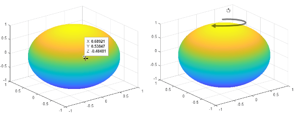
Two spheres created with approximately 800,000 scattered points. The first sphere shows a data tip and its marker, and the second shows the cursor in rotation mode.

Plots in Apps: Improved performance for creating plots

The performance is improved for creating plots in apps or in figures created with the uifigure function. For example, create a figure and an axes object. Then plot 10,000 points. This code runs 14x faster in R2021b.

function timingPlot
% Create figure and axes
f = uifigure;
ax = axes(f);
drawnow;

% Create data vector
y = rand(1,10000);

% Plot the data
tic;
plot(ax,y);
toc;
end

The approximate execution times are:

R2021a: 0.14 s

R2021b: 0.01 s

The code was timed on a Windows 10, Intel Xeon W-2133 CPU @ 3.60 GHz test system by calling the timingPlot function.

App Designer: Improved performance when opening Start Page and loading apps

When you use App Designer, these operations have improved performance:

  • Opening the App Designer Start Page

  • Opening an existing app

For example, opening App Designer by entering appdesigner in the Command Window loads the Start Page approximately 1.8x faster in R2021b than in R2021a the first time it is opened, and 2.1x faster in subsequent times. The approximate startup times are:

ReleaseFirst StartupSubsequent Startups
R2021a6.6 s3.6 s
R2021b3.6 s1.7 s

Also, loading an app in App Designer shows improved performance. For example, after creating and saving a new blank app, opening the app in App Designer is about 1.3x faster in R2021b than in R2021a. The approximate loading times are:

R2021a: 1.98 s

R2021b: 1.56 s

The performance improvement is larger if you have additional toolboxes installed.

These operations were timed on a Windows 10, Intel Core i7-5600 CPU @ 2.60 GHz test system.

App Designer: Improved performance when saving apps

Saving apps in App Designer after you edit an app function or property is faster in R2021b than in R2021a. The more lines of code in the app file, the greater the performance improvement becomes.

For example, on a Windows 10, Intel Xeon W-2133 CPU @ 3.60 GHz test system, in an app containing 10,000 lines of code, if you click Property to create a new property and then click Save to save the app, you can run the updated app sooner in R2021b than in R2021a.

The approximate save times are:

R2021a: 20 s

R2021b: 1.5 s

Comparison Tool: Improved performance when loading and saving MLAPP files

When you use the Comparison Tool to compare and merge changes between app code in MLAPP files, these operations have improved performance:

  • Loading the files into the Comparison Tool

  • Saving the files after merging changes

For example, if you load two apps with 5000 lines of code into the Comparison Tool by clicking Compare in the App Designer toolstrip, you can compare and merge the files sooner in R2021b than in R2021a.

The approximate loading times are:

R2021a: 13 s

R2021b: 8 s

Also, if you use the Comparison Tool to merge changes between two apps with 5000 lines of code (for example, by clicking Merge Mode , merging the changes, and then clicking Save Result ), you can compare the saved files sooner in R2021b than in R2021a.

The approximate save times are:

R2021a: 24 s

R2021b: 8 s

Both of these operations were timed on a Windows 10, Intel Xeon W-2133 CPU @ 3.60 GHz test system.

uigridlayout Function: Improved performance when adding components spanning multiple columns with 'fit' width

The performance of parenting components to a grid layout manager created using the uigridlayout function has improved when the components span multiple columns with a ColumnWidth value of 'fit'. The performance improvement gets better as the number of components spanning multiple columns and the number of columns spanned increases.

For example, this code creates a grid layout manager with 10 columns with a ColumnWidth value of 'fit', and then creates 50 labels that span all 10 columns. Performance in R2021b is about 4.7x faster than in R2021a.

function timingGridLayout
f = uifigure;
numrows = 50;
numcols = 10;
g = uigridlayout(f);
g.Scrollable = 'on';
g.RowHeight = repmat({'fit'},1,numrows);
g.ColumnWidth = repmat({'fit'},1,numcols);
drawnow

tic
for row = 1:numrows
    txt = ['This is a label in row ' num2str(row) ' that spans ' ...
        num2str(numcols) ' columns in the grid.'];
    lbl = uilabel(g,'Text',txt);
    lbl.Layout.Column = [1 numcols];
end
drawnow
toc
end

The approximate execution times are:

R2021a: 5.2 s

R2021b: 1.1 s

The code was timed on a Windows 10, Intel Xeon CPU E5-1650 v4 @ 3.60 GHz test system by calling the function timingGridLayout.

uigridlayout Function: Improved resizing performance when wrapping text in resizable columns

The performance when you resize apps containing a grid layout manager created using the uigridlayout function has improved when both of these conditions hold:

  • The grid layout manager contains a component with a WordWrap value of 'on'.

  • The row and column containing the component with word wrap have a RowHeight of 'fit' and a ColumnWidth that is resizable, such as '1x'.

For example, on a Windows 10, Intel Xeon CPU E5-1650 v4 @ 3.60 GHz test system, if you create 100 labels with wrapping text in a grid layout manager with fit height rows and resizable columns, and then resize the figure window by dragging the corner of the figure, the label text adjusts to fit the size of the figure almost immediately. In R2021a, there is a delay of about 2 seconds before the text adjusts.

f = uifigure;
g = uigridlayout(f);
g.ColumnWidth = {'1x'};
numrows = 100;
g.RowHeight = repmat({'fit'},numrows,1);
 
for row = 1:numrows
c = uilabel(g);
c.Text = ['Lorem ipsum dolor sit amet, consectetur adipiscing elit,' ...
' sed do eiusmod tempor incididunt ut labore et dolore magna aliqua.'];
c.WordWrap = 'on';
end
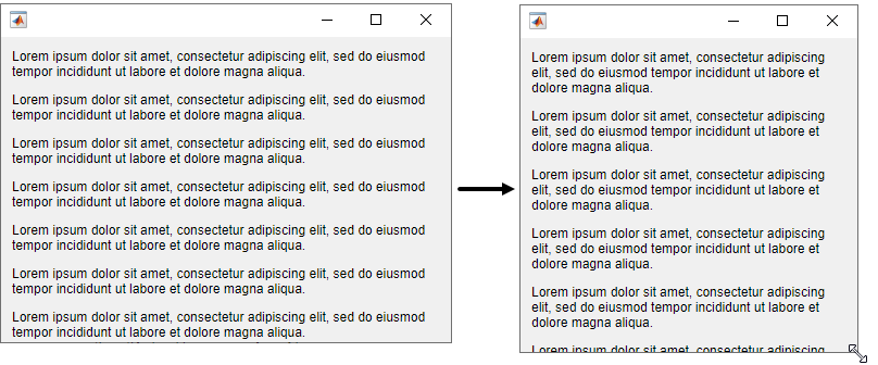
Two figure windows with labels with wrapping text. The right window is a resized version of the left window, where the wrapped label text takes up an additional row.

Live Editor: Improved performance when saving live scripts or functions

Saving live scripts and live functions in the Live Editor is faster in R2021b than in R2021a. The improvement is most noticeable when you save live functions with more than 1000 lines of code and live scripts with fewer than 100 lines of code.

For example, on a Windows 10, Intel Xeon E5-1650 CPU @ 3.60 GHz test system, saving an example live function containing 4000 lines of code takes approximately 2.05 seconds in R2021b. In R2021a, saving the same live function takes approximately 2.57 seconds.

Data Processing Dialog Boxes: Improved resizing performance

The Basic Fitting UI, Data Statistics UI, Colormap Editor, and Linked Plot Data Sources dialog now use uigridlayout to manage positions of UI components. This change results in a smoother experience when adjusting the size of these dialog boxes. For more information about the Data Statistics UI, see Computing with Descriptive Statistics.

For example, on a Windows 10, Intel Xeon E5-1650 CPU @ 3.60 GHz test system, when you increase the size of the Colormap Editor, the size changes smoothly.

Figure Interactions: Improved performance when using built-in axes interactions

Performance of figure interactions has been improved by coalescing built-in axes interactions so that there are significantly fewer interactions to process. These changes make interacting with a plot smoother and reduce the delay between an input and a response.

For example, on a Windows 10, Intel Xeon E5-1650 CPU @ 3.60 GHz test system, while panInteraction mode is active, when you click and drag the cursor within the axes the figure pans more quickly and tracks the cursor more closely.

UI Figures: Improved performance when displaying axes toolbar

The performance of the axes toolbar in UI figures has been improved to reduce the delay before the toolbar appears.

For example, on a Windows 10, Intel Xeon E5-1650 CPU @ 3.60 GHz test system, when you pause the cursor on the axes, the axes toolbar appears more quickly.

UI Figures: Improved performance when interacting with linked axes

Interacting with linked axes has improved performance when using figures created with the uifigure function or figures created in MATLAB Online™.

Software Development Tools

Projects: Collaborate using projects in MATLAB Online

Starting in R2021b, MATLAB Online provides support for basic projects workflows:

  • Create an empty project and add files and folders.

  • Clone a project from Git.

  • Explore your project and run a dependency analysis.

  • Create a project and manage your project files programmatically.

Source Control: Work with files under Git in MATLAB Online

Starting in R2021b, MATLAB Online provides support for basic Git workflows:

  • Cloning a remote Git repository

  • Committing files to Git

  • Pulling, pushing, and fetching files with Git

Unit Testing Framework: Use the TestCase class template to create tests more quickly and accurately

You can now create a TestCase class, including basic test functionality, in MATLAB and MATLAB Online. To create a new test class, select New > Test Class on the Home, Editor, or Live Editor tabs.

Use the TestCase class template to create tests more conveniently. The template includes a TestClassSetup methods block, a TestMethodSetup methods block, and a Test methods block that defines a simple Test method. To customize your test class, add code to the file or remove unused code that is included by default. For more information about class-based tests, see Author Class-Based Unit Tests in MATLAB.

Unit Testing Framework: Run live-function-based tests interactively in MATLAB Online

Starting in R2021b, you can run live-function-based tests interactively in MATLAB Online. When you open an MLX file defining a function-based test in MATLAB Online, the toolstrip lets you run all tests in the file or just the current test.

To run tests and customize your test run interactively, use the Run Tests section in the Live Editor tab of the toolstrip. For more information, see Run Tests in Editor.

App Testing Framework: Perform press gestures on axes and UI axes with different selection types

The app testing framework now supports mouse selection types in press gestures that are performed on axes and UI axes. For example, create an axes with a plot and then test a double-click gesture at the point (3, 2).

f = uifigure;
ax = axes(f);
plot(ax,1:10)
tc = matlab.uitest.TestCase.forInteractiveUse;
tc.press(ax,[3 2],'SelectionType','open')

App Testing Framework: Perform drag gestures on axes and figures with different selection types

Starting in R2021b, the app testing framework supports drag gestures on UI figures. Additionally, when you test a drag gesture on an axes, UI axes, or UI figure, you can specify the mouse selection type. For example, create a figure and drag on it from the point (100, 200) to the point (200, 300) using a right-click gesture.

f = uifigure;
tc = matlab.uitest.TestCase.forInteractiveUse;
tc.drag(f,[100 200],[200 300],'SelectionType','alt')

App Testing Framework: Use any units of measurement in gestures at the center of components

Starting in R2021b, when you perform a gesture at the center of a component, the component or its parent containers can use any units of measurement. In previous releases, the framework does not support containers that use nonpixel units.

For example, create a figure and set its Units property to 'normalized'. Then, create a panel in the figure and press at the center of the panel.

f = uifigure;
f.Units = 'normalized';
p = uipanel(f);
tc = matlab.uitest.TestCase.forInteractiveUse;
tc.press(p)

If you perform a gesture at the center of a component using a syntax that accepts location as an input (for instance, press(testcase,comp,location)), then the figure or parent containers can use only 'pixels' as their units of measurement.

 Functionality being removed or changed

Specifying diagnostic after name-value arguments in qualifications is not recommended

Still runs

Starting in R2021b, when you test for equality using the verifyEqual, assumeEqual, assertEqual, or fatalAssertEqual methods, specifying name-value arguments before the diagnostic input argument is not recommended. Place name-value arguments after all of the positional arguments instead. Although not recommended, you still can specify diagnostic after the name-value arguments when these arguments use the name,value syntax.

The reason for this change is that, starting in R2021a, MATLAB supports a new syntax for passing name-value arguments. In the new syntax, the name and value arguments are connected by an equals sign (name=value), and the name is not enclosed in quotes. To use the new syntax with qualification methods, specify positional arguments, including diagnostic, before the name=value arguments. If you specify diagnostic after name=value arguments, MATLAB produces an error.

This table shows an example of how you can update your code.

R2021a and EarlierStarting in R2021b
testCase = matlab.unittest.TestCase.forInteractiveUse;
verifyEqual(testCase,1.5,2, ...
    "RelTol",0.1,"Difference must be within relative tolerance.")
assumeEqual(testCase,1,2, ...
    "AbsTol",0.5,"Difference must be within absolute tolerance.")
testCase = matlab.unittest.TestCase.forInteractiveUse;
verifyEqual(testCase,1.5,2, ...
    "Difference must be within relative tolerance.",RelTol=0.1)
assumeEqual(testCase,1,2, ...
    "Difference must be within absolute tolerance.",AbsTol=0.5)

For more information, see verifyEqual.

matlab.unittest.TestSuite.fromProject ignores the files that do not define test procedures when creating a test suite

Behavior change

Starting in R2021b, if your project includes files with the Test classification, matlab.unittest.TestSuite.fromProject ignores the files that do not define test procedures when you create a test suite. For example, if an abstract TestCase class definition file is labeled with the Test classification, fromProject ignores it. In previous releases, MATLAB produces an error if fromProject is called on a project that uses the Test classification for any files other than concrete test files. With this change, fromProject becomes consistent with the matlab.unittest.TestSuite.fromFolder method: both methods create a test suite from all the concrete test files and ignore any other files in the folder.

This behavior change also applies to the testsuite, runtests, and runperf functions when they operate on code organized into files and folders within a project.

Test suites created from projects cannot run without the Java Virtual Machine (JVM) software

Behavior change

Starting in R2021b, if you start MATLAB without the Java Virtual Machine (JVM®) software and create a suite from the test files in a project using testsuite, the function uses the matlab.unittest.TestSuite.fromProject method to create the suite. If you then try to run the test suite without the JVM software, MATLAB produces an error because the project cannot be opened without the JVM software. In previous releases, when MATLAB runs without the JVM software, testsuite uses matlab.unittest.TestSuite.fromFolder to create a suite from the test files in the project, and the testing framework runs the resulting test suite.

This behavior change also applies to the runtests and runperf functions when they operate on code organized into files and folders within a project.

External Language Interfaces

C++ interface: Support for C++ language features

The C++ interface supports these additional C++ language features.

Support for void** parameters

MATLAB returns a void* argument for void** parameters. For more information, see void** Input Argument Types. For information about memory management of void** parameters, see Pass Ownership of Memory to MATLAB.

char [] parameters behave like char * parameters

MATLAB supports char[] parameters as either integer or character (string), the same as char* parameters. Likewise, the Unicode types wchar_t[], char16_t[], and char32_t[] behave like wchar_t*, char16_t*, and char32_t*. For more information, see C++ char* and char[] Types.

Support for static data members

Public static and public const static data members are treated as read-only properties in MATLAB. You cannot modify the value of a C++ static data member in MATLAB. For more information, see Static Data Members.

You can use a public static data member (property) as the data type of an input argument or return type in a class constructor, method, or function. You also can use a static property or method to define the shape of an argument. For information about using static properties to define the shape, see Use Property or Method as SHAPE.

C++ interface: Publisher options

The C++ interface supports these build configuration features.

Overwrite existing library definition files

Publishers can automatically overwrite existing library definition MLX files when calling clibgen.generateLibraryDefinition. Set the OverwriteExistingDefinitionFiles name-value argument to true. This option is useful when you create and modify the definition file for a library libname.

When you use this option, MATLAB deletes definelibname.mlx and definelibname.m, including any edits you made to the files.

Options for defining arguments

Java interface: Specify JRE path for MATLAB

You can run MATLAB with your system version of the Java Runtime Environment (JRE). For information about Java versions compatible with MATLAB, see MATLAB Interfaces to Other Languages.

To set the JRE path in MATLAB, call jenv. You must restart MATLAB to use the updated path. This command sets the path for all future MATLAB sessions but does not change the path for other applications on your computer.

Alternatively, you can set the path from the operating system prompt. Call matlab_jenv, then start MATLAB.

Java: Call into MATLAB from a Java program called by MATLAB

Java developers can use the com.mathworks.engine.MatlabEngine API getCurrentMatlab method to call back into MATLAB from Java. Incorporating this method in your application allows MATLAB users to call functionality from your Java program.

For information about developing these Java programs, see Call Back into MATLAB from Java.

Python interface: Run Python commands and scripts from MATLAB

The pyrun and pyrunfile functions let you call Python commands and scripts from MATLAB. For more information, see Directly Call Python Functionality from MATLAB

Python: Support for complex multidimensional arrays

MATLAB supports passing complex multidimensional array data to Python and from Python to MATLAB, for both in-process and out-of-process execution modes.​ For example, create a file test.py containing this code:

def returnData(data):
   return data

To pass a complex MATLAB array to returnData, type:

mc = complex(magic(3));
c = py.test.returnData(mc)
c = 
  Python memoryview:

   8.0000 + 0.0000i   1.0000 + 0.0000i   6.0000 + 0.0000i
   3.0000 + 0.0000i   5.0000 + 0.0000i   7.0000 + 0.0000i
   4.0000 + 0.0000i   9.0000 + 0.0000i   2.0000 + 0.0000i

    Use details function to view the properties of the Python object.

    Use double function to convert to a MATLAB array.

To convert the return value to a MATLAB array, type:

C = double(c)
C = 3×3 complex    
   8.0000 + 0.0000i   1.0000 + 0.0000i   6.0000 + 0.0000i
   3.0000 + 0.0000i   5.0000 + 0.0000i   7.0000 + 0.0000i
   4.0000 + 0.0000i   9.0000 + 0.0000i   2.0000 + 0.0000i

For information about MATLAB to Python data type mapping, see Pass Matrices and Multidimensional Arrays to Python.

Python: Version 3.9 support

MATLAB now supports CPython 3.9, in addition to existing support for 2.7, 3.7, and 3.8. For more information, see Versions of Python Compatible with MATLAB Products by Release

 WSDL Web Services Documents: Apache CXF version 3.4.2 support

MATLAB supports Apache CXF version 3.4.2 for use with WSDL Web services. For more information, see Set Up WSDL Tools.

 Compatibility Considerations

Download the latest version 3.4.2 release of the Apache CXF tool from https://cxf.apache.org/download.

 Perl 5.32.1: MATLAB support on Windows

As of R2021b, MATLAB on Windows ships with an updated version of Perl, version 5.32.1. See https://www.perl.org for a standard distribution of Perl, Perl source code, and information about using Perl.

 Compatibility Considerations

If you use the perl command on Windows platforms, see https://www.perl.org for information about using this version of the Perl programming language.

 Functionality being removed or changed

name=value syntax errors for calls to Python functions using py. prefix

Behavior change

Starting in R2021b, MATLAB errors when you use name=value syntax for passing keyword arguments to Python functions using the py. prefix. In R2021a, MATLAB might silently give the wrong answer. Use pyargs to pass keyword arguments.

For example, the Python print function has a keyword argument sep. This Python statement sets the sep argument to a comma followed by a space:

print('comma','separated','values',sep=', ')

When you call this statement in MATLAB, MATLAB interprets sep=', ' as a name=value argument:

py.print('comma','separated','values',sep=', ')
R2021a BehaviorR2021b BehaviorHow to Update Your Code

py.print(...
    'comma','separated','values',...
    sep=', ')
Silent wrong answer:
comma separated values sep , 

py.print(...
    'comma','separated','values',...
    sep=', ')
Error:
Error using py.print 
Using name=value format is not supported. 
Use pyargs to pass keyword arguments

py.print(...
    'comma','separated','values',...
    pyargs(sep=', '))
comma, separated, values

createSoapMessage, callSoapService, and parseSoapResponse have been removed

Errors

Consider using matlab.wsdl.createWSDLClient instead of the createSoapMessage, callSoapService, and parseSoapResponse functions to communicate with Web services using Simple Object Access Protocol (SOAP). There is no direct function replacement for the SOAP functions, but when you create a WSDL interface, you have access to the Web service functionality.

createClassFromWsdl has been removed

Errors

The matlab.wsdl.createWSDLClient function replaces the createClassFromWsdl function to communicate with Web services from MATLAB using Web Services Description Language (WSDL). matlab.wsdl.createWSDLClient enables you to specify additional information needed to access the WSDL document. For more information, see weboptions.

To get started using matlab.wsdl.createWSDLClient, follow these steps.

  1. Download supported versions of the Java JDK and Apache CXF programs. For more information, see Set Up WSDL Tools.

  2. Set the paths to these programs, where jdk is the path to the JDK installation and cxf is the path to the CXF program.

    matlab.wsdl.setWSDLToolPath('JDK',jdk,'CXF',cxf)

To update your code, replace calls to createClassFromWsdl with calls to matlab.wsdl.createWSDLClient. For example, for a Web service with this URL:

url = 'https://examplesite.com/samplewebservice';

replace this call to createClassFromWsdl:

createClassFromWsdl(strcat(url,'?WSDL'))

with:

matlab.wsdl.createWSDLClient(url)

Note

matlab.wsdl.createWSDLClient does not support RPC-encoded WSDL documents.

Hardware Support

Connect and Control Arduino board using the Arduino Explorer App

The MATLAB Support Package for Arduino Hardware now has an Arduino Explorer app.

Using this app, you can:

  • Set up the Arduino board

  • Connect to an Arduino board over USB, Bluetooth, and WiFi

  • Configure, read from, and write to Arduino pins

  • Visualize data from Arduino pins

  • Record and save data from Arduino pins to the MATLAB workspace

  • Analyze the recorded data

  • Generate equivalent MATLAB code

Read data from APDS9960 sensor connected to the Arduino hardware

The MATLAB Support Package for Arduino Hardware enables you to read gesture, proximity, clear light and color (RGB) data from APDS9960 sensor connected to Arduino hardware.

Support for CAN shields on Raspberry Pi Hardware

Use the Raspberry Pi Blockset to read and write CAN messages from the CAN network on the Raspberry Pi hardware.