Results for



20 minutes makes a difference

I struggled to learn MATLAB at first. A colleague at my university gave me about 20 minutes of his time to show me some basic features, how to reference the documentation, and how to debug code. That was enough for me to start using MATLAB independently. After a few semesters of developing analyses and visualizations, I started answering questions in the forum when I had time. I became addicted to volunteering and learning from the breadth of analytical problems the forum exposed me to.



Have you ever solved a problem using a MathWorks product?

If your answer is YES, you may be the right person to help someone looking for guidance to solve a similar problem. Some answers in the MATLAB Central community forum maintain 1000s of views per month and some files on the File Exchange have 1000s of downloads. Volunteering a moment of your time to answer a question or to share content to the File Exchange may benefit countless individuals in the near and distant future and you will likely learn a lot by contributing too!

• 3616 questions were asked last month in the forum and in that time, 747 volunteers answered at least one question!
• 62% of those volunteers were first-time contributors!
• 335 volunteer contributors shared content in the File Exchange last month!
• 1: the number of contributions it takes to make a difference.

This week is National Volunteer Week in the USA (April 17-23). Challenge yourself and your colleagues by committing to help a stranger break barriers in their path to learning MATLAB.



How to volunteer and contribute to the MATLAB Central Community

Here are two easy ways to accept the volunteer challenge.

Contribute to the MATLAB Answers Forum

1. Go to the MATLAB Answers repository. This page shows all unanswered questions starting with the most recent question. Use the filters on the left to see answered questions or questions belonging to a specific category. Alternatively, search for questions using keywords in the search field or visit the landing page.
2. Open a few questions that interest you based on the question titles and tags.
3. Decide how you'd like to contribute. Sometimes a question needs refinement or requires a bit of work to address. Decide whether to leave a comment that guides the user in the right direction, answer the question, or skip to the next question. The decision tree below is how some experienced contributors approach these decisions.

Pro tips

• Newer questions have more traffic and are often answered within an hour or minutes.
• Multiple answers often add valuable alternative perspectives and solutions.
• Sometimes answers aren't accepted or the asker disappears. Be not discouraged. Your answer holds much value.



Contribute to the File Exchange

1. Choose a function, script, demo, or toolbox you created that may be helpful to the community.
2. Go to the MathWorks File Exchange. Search for submissions that are similar to your idea and decide whether your idea adds value.
3. Prepare your code for open-source sharing. The best submissions include brief documentation that explains the purpose of the code, inputs, expected outputs and limitations.
4. Use the "Publish your code" button from the link above. This will guide you through the submission process.



Make a difference

No matter what level you are at as a MATLAB developer, you have skills that others around you could benefit from learning. Take the challenge and become a giant.

Let us know about your experience with MATLAB Central volunteers or your experience becoming a MATLAB Central volunteer in the comments below!

.

MATLAB R2022a provides app developers more control over user navigation through app components using the keyboard's Tab key.

Part 1. The new focus function: programmatically set keyboard focus to a UI component

Part 2. Modify focus order of components

Today we'll review Part 2. See yesterday's Community Highlight for Part 1.

-------------------------------------------------------------------------------------------------

Well-designed apps have an obvious flow through interactive fields and, as we learned yesterday, using the Tab key to move the focus to the next UI component is faster and more efficient than using a mouse. Here we'll learn how to read and set the tab order of UI components in an app.

Understanding tab and stacking order

By default, tab order in MATLAB apps is controlled by the stacking order in the Component Browser. Initially, the stacking order within the component browswer is based on the sequence in which the objects were added to the container object within the app. MATLAB R2020b gave us control to edit the stacking order by selecting a component and using either the Reorder tool from the Canvas toolstrip or by right-clicking the component and selecting Reorder from the context menu [1]. Tab order flows from bottom to top through the Component Browswer hierarchy for objects that are focusable. Sending a component backward within the stack sets its tab order to earlier relative to other components.

Setting tab focus order in R2022a

Three additional tab order features were added in MATLAB R2022a that make it easier to control app navigation with the Tab key.

1. Sort and Filter by Tab Order : Instead of using the Reorder tool which lists components in reverse tab-order and includes components that are not focusable, filter the list by focusable components and sort them by tab-order using the View dropdown menu within the Component Browser (label 1 in image below). From here, you can drag and drop components to set their tab (and stacking) order.

2. Auto Tab Order : To automatically sort focusable components within your app so that the tab order is from left-to-right and then top-to-bottom, in App Designer, from Design View, select the Canvas tab > Tab Order button > Apply Auto Tab Order (label 2 in image below). Alternatively, you can apply auto tab order to components within a container such as a uipanel or uitab by right-clicking on the container within the Component Browser and selecting Apply Auto Tab Order.

3. Visualize Tab Order : You no longer have to read and interpret the handle names in the component browser to understand the current tab order of UI components. Instead, view an animation of tab order within App Designer. From Design View, select the Canvas tab > Tab Order button > Visualize Tab Order (label 3 in image below).

.

Contextual focus control: the power of combining focus() with setting tab order

Yesterday's Community Highlight showed how to programmatically set UI component focus using the focus(c) function. This, combined with control of tab order, allows app developers to implement contextual focus control. For example, when a radio button is selected in the GIF below, the corresponding UI Tab is selected programmatically and the keyboard focus is set to the first component within the UI Tab thus allowing the user to smoothly continue keyboard navigation. This is achieved by a callback function that responds to changes in the Button Group that sets the SelectedTab property of the TabGroup and uses the new focus() function. For details, see the attached focusAndTabOrderDemo.mlapp.

-------------------------------------------------------------------------------------------------

Stay tuned

Follow Community Highlights to get notifications for new content.

Let us know what interests you in the new MATLAB R2022a release in the comment section below.

See also

• MATLAB documentation: Modify Tab Focus Order of Components
• Release notes: Modify tab focus order
• R2021a Highlight: keyboard shortcuts for UI Components
• Download the latest release of MATLAB

Footnotes

[1] R202b release notes: change the stacking order of UI components

This Community Highlight is attached as a live script.

.

MATLAB R2022a provides app developers more control over user navigation through app components using the keyboard's Tab key.

Part 1. The new focus function: programmatically set keyboard focus to a UI component

Part 2. Modify focus order of components

Today we'll review Part 1. Come back tomorrow for Part 2.

-------------------------------------------------------------------------------------------------

Programmatically set UI component focus

Did you know that you can save ~2 seconds every time you use a keyboard shortcut rather than reaching for your mouse [1,2]?

I need you to focus here: starting in MATLAB R2022a, use the new focus function to set keyboard focus to a specific UI component.

By specifying the component handle ( c ) in focus(c),

1. The figure containing the component is displayed
2. A blue frame appears around the component
3. The user can directly interact with the component.

.

Which components are focusable?

Focusable components are those that a user can interact with using the keyboard. So an object set to Enable='off' or Visible='off' cannot be in focus. See the documentation for more details.

What will you do with all of that extra time saved?

-------------------------------------------------------------------------------------------------

Stay tuned

Tomorrow we'll learn how to apply the new focus function with control of tab order to create contextual flow of UI component focus. Follow Community Highlights to get notifications.

Let us know what interests you in the new MATLAB R2022a release in the comment section below.

See also

• Release notes: focus
• R2021a Highlight: keyboard shortcuts for UI Components
• Download the latest release of MATLAB

Footnotes

[1] Lane et. al. (2005). International Journal of Human-Computer Interaction, 18(2).

[2] Michels (2018). median.com

This Community Highlight is attached as a live script.

Starting in MATLAB R2022a, use the append option in exportgraphics to create GIF files from animated axes, figures, or other visualizations.

This basic template contains just two steps:

% 1. Create the initial image file
gifFile = 'myAnimation.gif';
exportgraphics(obj, gifFile);

% 2. Within a loop, append the gif image
for i = 1:20

      %   %   %   %   %   %    % 
      % Update the figure/axes %
      %   %   %   %   %   %    % 

      exportgraphics(obj, gifFile, Append=true);
  end

Note, exportgraphics will not capture UI components such as buttons and knobs and requires constant axis limits.

To create animations of images or more elaborate graphics, learn how to use imwrite to create animated GIFs .

Share your MATLAB animated GIFs in the comments below!

See Also

• Animation Techniques
• Animating plots

This Community Highlight is attached as a live script

You've spent hours designing the perfect figure and now it's time to add it to a presentation or publication but the font sizes in the figure are too small to see for the people in the back of the room or too large for the figure space in the publication. You've got titles, subtitles, axis labels, legends, text objects, and other labels but their handles are inaccessible or scattered between several blocks of code. Making your figure readable no longer requires digging through your code and setting each text object's font size manually.

Starting in MATLAB R2022a, you have full control over a figure's font sizes and font units using the new fontsize function (see release notes ).

Use fontsize() to

• Set FontSize and FontUnits properties for all text within specified graphics objects
• Incrementally increase or decrease font sizes
• Specify a scaling factor to maintain relative font sizes
• Reset font sizes and font units to their default values . Note that the default font size and units may not be the same as the font sizes/units set directly with your code.

When specifying an object handle or an array of object handles, fontsize affects the font sizes and font units of text within all nested objects.

While you're at it, also check out the new fontname function that allows you to change the font name of objects in a figure!

Give the new fontsize function a test drive using the following demo figure in MATLAB R2022a or later and try the following commands:

% Increase all font sizes within the figure by a factor of 1.5
fontsize(fig, scale=1.5)

% Set all font sizes in the uipanel to 16
fontsize(uip, 16, "pixels")

% Incrementally increase the font sizes of the left two axes (x1.1)
% and incrementally decrease the font size of the legend (x0.9)
fontsize([ax1, ax2], "increase")
fontsize(leg, "decrease")

% Reset the font sizes within the entire figure to default values
fontsize(fig, "default")

% Create fake behavioral data
rng('default')
fy = @(a,x)a*exp(-(((x-8).^2)/(2*3.^2)));
x = 1 : 0.5 : 20;
y = fy(32,x);
ynoise = y+8*rand(size(y))-4;
selectedTrial = 13;

% Plot behavioral data
fig = figure('Units','normalized','Position',[0.1, 0.1, 0.4, 0.5]);
movegui(fig, 'center')
tcl = tiledlayout(fig,2,2); 
ax1 = nexttile(tcl); 
hold(ax1,'on')
h1 = plot(ax1, x, ynoise, 'bo', 'DisplayName', 'Response');
h2 = plot(ax1, x, y, 'r-', 'DisplayName', 'Expected');
grid(ax1, 'on')
title(ax1, 'Behavioral Results')
subtitle(ax1, sprintf('Trial %d', selectedTrial))
xlabel(ax1, 'Time (seconds)','Interpreter','Latex')
ylabel(ax1, 'Responds ($\frac{deg}{sec}$)','Interpreter','Latex')
leg = legend([h1,h2]);

% Plot behavioral error
ax2 = nexttile(tcl,3);
behavioralError = ynoise-y; 
stem(ax2, x, behavioralError)
yline(ax2, mean(behavioralError), 'r--', 'Mean', ...
    'LabelVerticalAlignment','bottom')
grid(ax2, 'on')
title(ax2, 'Behavioral Error')
subtitle(ax2, ax1.Subtitle.String)
xlabel(ax2, ax1.XLabel.String,'Interpreter','Latex')
ylabel(ax2, 'Response - Expected ($\frac{deg}{sec}$)','Interpreter','Latex')

% Simulate spike train data
ntrials = 25; 
nSamplesPerSecond = 3; 
nSeconds = max(x) - min(x); 
nSamples = ceil(nSeconds*nSamplesPerSecond);
xTime = linspace(min(x),max(x), nSamples);
spiketrain = round(fy(1, xTime)+(rand(ntrials,nSamples)-.5));
[trial, sample] = find(spiketrain);
time = xTime(sample);

% Spike raster plot
axTemp = nexttile(tcl, 2, [2,1]);
uip = uipanel(fig, 'Units', axTemp.Units, ...
    'Position', axTemp.Position, ...
    'Title', 'Neural activity', ...
    'BackgroundColor', 'W');
delete(axTemp)
tcl2 = tiledlayout(uip, 3, 1);
pax1 = nexttile(tcl2); 
plot(pax1, time, trial, 'b.', 'MarkerSize', 4)
yline(pax1, selectedTrial-0.5, 'r-', ...
    ['\leftarrow Trial ',num2str(selectedTrial)], ...
    'LabelHorizontalAlignment','right', ...
    'FontSize', 8); 
linkaxes([ax1, ax2, pax1], 'x')
pax1.YLimitMethod = 'tight';
title(pax1, 'Spike train')
xlabel(pax1, ax1.XLabel.String)
ylabel(pax1, 'Trial #')

% Show MRI
pax2 = nexttile(tcl2,2,[2,1]); 
[I, cmap] = imread('mri.tif');
imshow(I,cmap,'Parent',pax2)
hold(pax2, 'on')
th = 0:0.1:2*pi; 
plot(pax2, 7*sin(th)+84, 5*cos(th)+90, 'r-','LineWidth',2)
text(pax2, pax2.XLim(2), pax2.YLim(1), 'ML22a',...
    'FontWeight', 'bold', ...
    'Color','r', ...
    'VerticalAlignment', 'top', ...
    'HorizontalAlignment', 'right', ...
    'BackgroundColor',[1 0.95 0.95])
title(pax2, 'Area of activation')

% Overall figure title
title(tcl, 'Single trial responses')

This Community Highlight is attached as a live script.

Starting in MATLAB R2021a axis tick labels will auto-rotate to avoid overlap when the user manually specifies ticks or tick labels ( release notes ). In custom visualization functions, the tick label density or tick label lengths may be variable and unknown. The new auto-rotation feature removes the burden of detecting the need to rotate manually-set labels and eliminates the need to manually rotate them.

Many properties and combinations of properties can cause tick labels to overlap if they are not rotated.

• Length of tick labels
• Number of tick labels
• Interval between tick labels
• Font size
• Font name
• Figure size
• Axes size
• Viewing angle of the axes

Demo: varying tick density and length of tick labels

These 9 axes vary by the number of x-ticks and length of x-tick-labels. MATLAB auto-rotates the labels when needed.

Demo: Changes to axis view angle and rotation

The auto-rotation feature updates the label angles as the axes change programmatically or during user interaction.

What if I don't want auto-rotation?

Auto-rotation mode is on by default for each X|Y|Z axis. When the tick label rotation angle is manually set from the X|Y|ZTickLabelRotation property of axes or by using xtickangle | ytickangle | ztickangle , auto-rotation is turned off. Auto-rotation can also be turned off by setting the X|Y|ZTickLabelRotationMode axis property to manual but it's important to also hold the axis properties so that the rotation mode does not revert to the default value, auto. If you're looking for a broader method of reverting to older behavior you can set the default label rotation mode to manual at the start of a function that produces multiple plots and then revert to the factory default rotation mode at the end of the file (consider using onCleanup).

set(groot,'defaultAxesXTickLabelRotationMode','manual')
set(groot,'defaultAxesYTickLabelRotationMode','manual')
set(groot,'defaultAxesZTickLabelRotationMode','manual')

% Revert to factory-default
set(groot,'defaultAxesXTickLabelRotationMode','remove')
set(groot,'defaultAxesYTickLabelRotationMode','remove')
set(groot,'defaultAxesZTickLabelRotationMode','remove')

A copy of this Community Highlight is attached as a live script.

Four (of many) new features for Apps in MATLAB R2021a

These four new features are the solutions to many inquiries in the Answers forum that continue to receive hundreds of views per month long after they were asked.

Table of Contents

• Keyboard Shortcuts for UI Components
• Programmatically scroll UITables
• Figure always on top
• UI hyperlink component
• Demo app: Keyboard shortcut challenge

Keyboard Shortcuts for UI Components

Keyboard shortcuts can now change the focus and make contiguous and non-contiguous selections in ListBox, Table, DatePicker, and ColorPicker menus created in uifigures. The table below summarizes the shortcuts made available in R2021a ( release notes ).

Reminder: in MATLAB R2020b and later you can change the tab order of objects in an app by changing their stack order in AppDesigner using the Reorder tool in the drop-down menu or by right-clicking the component and selecting Reorder from the menu (see R2020b release notes and a screenshot in the Answers forum ).

Programmatically scroll UITables

The scroll function was added in R2016a but as of R2021a it can be used with uitables to programmatically scroll to the top, bottom, left, or right of a table or to a specific row, column or cell ( release notes ). Combined with a uistyle (R2019b) you can scroll to and highlight any part of the uitable.

Syntax examples:

• scroll(uit,vlocation) where vlocation is 'top'-'bottom'
• scroll(uit,hlocation) where hlocation is 'left'-'right'
• scroll(uit,target,targetIndex) where target is 'row'-'column'-'cell' and targetIndex is a row or column number or a 1x2 cell location.

Figure always on top

Figures created with uifigure now have an additional WindowStyle property: 'alwaysontop' ( release notes ). Figures with this setting will stay on top of other windows but unlike the modal option, other windows are still accessible.

See the WindowStyle property description for tips on setting and changing this property.

To toggle the AlwaysOnTop state of your app using a checkbox, state button, or another UI component, follow this callback function template,

function alwaysOnTopCheckBoxValueChanged(app, event)
    value = app.alwaysOnTopCheckBox.Value;
    if value
        app.UIFigure.WindowStyle = 'alwaysontop';
    else
        app.UIFigure.WindowStyle = 'normal';
    end
end

UI hyperlink component

Use the uihyperlink function or the UI hyperlink component in App Designer or a uifigure to add and configure a clickable link ( release notes ). The hyperlink can be assigned to a figure, panel object, tab object, ButtonGroup, or GridLayout object when created in a uifigure. In addition to setting the text and URL, there are lots of properties to control the text format including the VisitedColor property that controls the color of the text after the link is clicked and an optional user-defined HyperlinkClickedFcn function that is evoked when the link is clicked.

Demo app: Keyboard shortcut challenge

The attached zip file contains an app, keyboardShortcutsDemo_R2021a.mlapp , that demonstrates these 4 features. The app displays the extent of arctic sea ice from 1979 to 2016 during the months when extent typically maximizes and minimizes.

Mouseless challenge: After opening the app, without using your mouse, try the following.

• Select a month (September or March) and any number of years from the list boxes
• Navigate through the Date Picker and select a date within the range or your selected years (disabled when only 1 year is selected).
• Navigate to the always-on-top checkbox to pin the app to the top of other windows.
• Navigate to the text box and enter a year that appears in the uitable to go to that row in the uitable (disabled when only 1 year is selected).
• Navigate to the URL and press Enter to open the website containing the raw data.

Download the attached zip file, FourNewAppFeatures_R2021a.zip, for a Live script copy of this thread and an app that demonstrates each feature.

New in R2021a, LimitsChangedFcn

LimitsChangedFcn is a callback function that responds to changes to axis limits ( release notes ). The function responds to axis interaction such as panning and zooming, programmatically setting the axis limits, or when axis limits are automatically adjusted by other processes.

LimitsChangedFcn is a property of ruler objects which are properties of axes and can be independently set for each axis. For example,

ax = gca(); 
ax.XAxis.LimitsChangedFcn = ... % Responds to changes to XLim
ax.YAxis.LimitsChangedFcn = ... % Responds to changes to YLim
ax.ZAxis.LimitsChangedFcn = ... % Responds to changes to ZLim

Previously, a listener could be assigned to respond to changes to axis limits. Here are some examples.

• Update refline when axis limits change
• Update axis2 limits when axis1 limits change

However, LimitsChangedFcn responds more reliably than a listener that responds to setting/getting axis limits. For example, after zooming or panning the axes in the demo below, the listener does not respond to the Restore View button in the axis toolbar but LimitsChangedFcn does! After restoring the view, try zooming out which does not result in changes to axis limits yet the listener will respond but the LimitsChangedFcn will not. Adding objects to axes after an axis-limit listener is set will not trigger the listener even if the added object expands the axis limits ( why not? ) but LimitsChangedFcn will!

ax = gca(); 
ax.UserData.Listener = addlistener(ax,'XLim','PostSet',@(~,~)disp('Listener')); 
ax.XAxis.LimitsChangedFcn = @(~,~)disp('LimitsChangedFcn')

How to use LimitsChangedFcn

The LimitsChangedFcn works like any other callback. For review,

• Callback Definition
• Write Callbacks for Apps

The first input to the LimitsChangedFcn callback function is the handle to the axis ruler object that was changed.

The second input is a structure that contains the old and new limits. For example,

    LimitsChanged with properties:

      OldLimits: [0 1]
      NewLimits: [0.25 0.75]
         Source: [1×1 NumericRuler]
      EventName: 'LimitsChanged'

Importantly, since LimitsChangedFcn is a property of the axis rulers rather than the axis object, changes to the axes may clear the LimitsChangedFcn property if the axes aren't held using hold on. For example,

% Axes not held
ax = gca(); 
ax.XAxis.LimitsChangedFcn = @(ruler,~)title(ancestor(ruler,'axes'),'LimitsChangedFcn fired!'); 
plot(ax, 1:5, rand(1,5), 'o')
ax.XAxis.LimitsChangedFcn

ans =
    0×0 empty char array

% Axes held
ax = gca(); 
hold(ax,'on')
ax.XAxis.LimitsChangedFcn = @(ruler,~)title(ancestor(ruler,'axes'),'LimitsChangedFcn fired!'); 
plot(ax, 1:5, rand(1,5), 'o')
ax.XAxis.LimitsChangedFcn

ans =
  function_handle with value:
    @(ruler,~)title(ancestor(ruler,'axes'),'LimitsChangedFcn fired!')

Demo

In this simple app a LimitsChangedFcn callback function is assigned to the x and y axes. The function does two things:

1. Text boxes showing the current axis limits are updated
2. The prying eyes that are centered on the axes will move to the new axis center

This demo also uses Name=Value syntax and emoji text objects !

Create app

h.fig = uifigure(Name="LimitsChangedFcn Demo", ...
    Resize="off");
h.fig.Position(3:4) = [500,260];
movegui(h.fig)
h.ax = uiaxes(h.fig,...
    Units="pixels", ...
    Position=[200 26 250 208], ...
    Box="on");
grid(h.ax,"on")
title(h.ax,"I'm following you!")
h.eyeballs = text(h.ax, .5, .5, ...
    char([55357 56385 55357 56385]), ...
    HorizontalAlignment="center", ...
    FontSize=40);
h.label = uilabel(h.fig, ...
    Text="Axis limits", ...
    Position=[25 212 160 15], ...
    FontWeight="bold",...
    HorizontalAlignment="center");
h.xtxt = uitextarea(h.fig, ...
    position=[25 191 160 20], ...
    HorizontalAlignment="center", ...
    WordWrap="off", ...
    Editable="off",...
    FontName=get(groot, 'FixedWidthFontName'));
h.ytxt = uitextarea(h.fig, ...
    position=[25 165 160 20], ...
    HorizontalAlignment="center", ...
    WordWrap="off", ...
    Editable="off", ...
    FontName=get(groot, 'FixedWidthFontName'));
h.label = uilabel(h.fig, ...
    Text=['X',newline,newline,'Y'], ...
    Position=[10 170 15 38], ...
    FontWeight="bold");

Set LimitsChangedFcn of x and y axes

h.ax.XAxis.LimitsChangedFcn = @(hObj,data)limitsChangedCallbackFcn(hObj,data,h,'x');
h.ax.YAxis.LimitsChangedFcn = @(hObj,data)limitsChangedCallbackFcn(hObj,data,h,'y');

Update text fields

xlim(h.ax, [-100,100])
ylim(h.ax, [-100,100])

Define LimitsChangedFcn

function limitsChangedCallbackFcn(rulerHand, limChgData, handles, xy)
% limitsChangedCallbackFcn() responds to changes to x or y axis limits.
% - rulerHand: Ruler handle for x or y axis that was changed (not used in this demo)
% - limChgData: LimitsChanged data structure
% - handles: structure of App handles
% - xy: either 'x' or 'y' identifying rulerHand
switch lower(xy)
    case 'x'
        textHandle = handles.xtxt;
        positionIndex = 1; 
    case 'y'
        textHandle = handles.ytxt;
        positionIndex = 2; 
    otherwise
        error('xy is a character ''x'' or ''y''.')
end
% Update text boxes showing rounded axis limits
textHandle.Value = sprintf('[%.3f, %.3f]',limChgData.NewLimits);
% Move the eyes to the new center position
handles.eyeballs.Position(positionIndex) = limChgData.NewLimits(1)+range(limChgData.NewLimits)/2; % for linear scales only!
drawnow
end

See attached mlx file for a copy of this thread.

Highlight Icon image

Starting in MATLAB R2021a, name-value arguments have a new optional syntax!

A property name can be paired with its value by an equal sign and the property name is not enclosed in quotes.

Compare the comma-separated name,value syntax to the new equal-sign syntax, either of which can be used in >=r2021a:

• plot(x, y, "b-", "LineWidth", 2)
• plot(x, y, "b-", LineWidth=2)

It comes with some limitations:

1. It's recommended to use only one syntax in a function call but if you're feeling rebellious and want to mix the syntaxes, all of the name=value arguments must appear after the comma-separated name,value arguments.
2. Like the comma-separated name,value arguments, the name=value arguments must appear after positional arguments.
3. Name=value pairs must be used directly in function calls and cannot be wrapped in cell arrays or additional parentheses.

Some other notes:

1. The property names are not case-sensitive so color='r' and Color='r' are both supported.
2. Partial name matches are also supported. plot(1:5, LineW=4)

The new syntax is helpful in distinguishing property names from property values in long lists of name-value arguments within the same line.

For example, compare the following 2 lines:

h = uicontrol(hfig, "Style", "checkbox", "String", "Long", "Units", "Normalize", "Tag", "chkBox1")

h = uicontrol(hfig,  Style="checkbox",    String="Long",    Units="Normalize",    Tag="chkBox1")

Here's another side-by-side comparison of the two syntaxes. See the attached mlx file for the full code and all content of this Community Highlight.

tiledlayout, introduced in MATLAB R2019b, offers a flexible way to add subplots, or tiles, to a figure.

Reviewing two changes to tiledlayout in MATLAB R2021a

1. The new TileIndexing property
2. Changes to TileSpacing and Padding properties

1) TileIndexing

By default, axes within a tiled layout are created from left to right, top to bottom, but sometimes it's better to organize plots column-wise from top to bottom and then left to right. Starting in r2021a, the TileIndexing property of tiledlayout specifies the direction of flow when adding new tiles.

tiledlayout(__,'TileIndexing','rowmajor') creates tiles by row (default).

tiledlayout(__,'TileIndexing','columnmajor') creates tiles by column.

.

2) TileSpacing & Padding changes

Some changes have been made to the spacing properties of tiles created by tiledlayout.

TileSpacing: sets the spacing between tiles.

• "loose" is the new default and replaces "normal" which is no longer recommended but is still accepted.
• "tight" replaces "none" and brings the tiles closer together still leaving space for axis ticks and labels.
• "none" results in tile borders touching, following the true meaning of none.
• "compact" is unchanged and has slightly more space between tiles than "tight".

Padding: sets the spacing of the figure margins.

• "loose" is the new default and replaces "normal" which is no longer recommended but is still accepted.
• "tight" replaces "none" and reduces the figure margins. "none" is no longer recommended but is still accepted.
• "compact" is unchanged and adds slightly more marginal space than "tight".
• Reducing the figure margins to a true none is still not an option.

The release notes show a comparison of these properties between r2020b and r2021a.

Here's what the new TileSpacing options (left column of figures below) and Padding options (right column) look like in R2021a. Spacing properties are written in the figure names.

.

And here's a grid of all 12 combinations of the 4 TileSpacing options and 3 Padding options in R2021a.

.

Code used to generate these figures

%% Animate the RowMajor and ColumnMajor indexing with colored tiles 
fig1 = figure('position',[200 200 560 420]); 
tlo1 = tiledlayout(fig1, 3, 3, 'TileIndexing','rowmajor');
title(tlo1, 'RowMajor indexing')

fig2 = figure('position',[760 200 560 420]); 
tlo2 = tiledlayout(fig2, 3, 3, 'TileIndexing','columnmajor');
title(tlo2, 'ColumnMajor indexing')

colors = jet(9);
drawnow()

for i = 1:9
    ax = nexttile(tlo1);
    ax.Color = colors(i,:);
    text(ax, .5, .5, num2str(i), 'Horiz','Cent','Vert','Mid','Fontsize',24)

      ax = nexttile(tlo2);
      ax.Color = colors(i,:);
      text(ax, .5, .5, num2str(i), 'Horiz','Cent','Vert','Mid','Fontsize',24)

      drawnow
      pause(.3)
  end

%% Show TileSpacing options
tileSpacing = ["loose","compact","tight","none"];
figHeight = 140;  % unit: pixels
figPosY = fliplr(50 : figHeight+32 : (figHeight+30)*numel(tileSpacing)); 

for i = 1:numel(tileSpacing)
    uif = uifigure('Units','Pixels','Position', [150 figPosY(i) 580 figHeight], ...
        'Name', ['TileSpacing: ', tileSpacing{i}]);
    tlo = tiledlayout(uif,1,3,'TileSpacing',tileSpacing(i)); 
    h = arrayfun(@(i)nexttile(tlo), 1:tlo.GridSize(2));
    box(h,'on')
    drawnow()
end

%% Show Padding options
padding = ["loose","compact","tight"];
for i = 1:numel(padding)
    uif = uifigure('Units','Pixels','Position', [732 figPosY(i) 580 figHeight], ...
        'Name', ['Padding: ', padding{i}]);
    tlo = tiledlayout(uif,1,3,'Padding',padding(i)); 
    h = arrayfun(@(i)nexttile(tlo), 1:tlo.GridSize(2));
    box(h,'on')
    drawnow()
end

%% Show all combinations of TileSpacing and Padding options
tileSpacing = ["loose","compact","tight","none"];
padding = ["loose","compact","tight"];
[tsIdx, padIdx] = meshgrid(1:numel(tileSpacing), 1:numel(padding));
figSize = [320 220]; % width, height (pixels)
figPosX = 150 + (figSize(1)+2)*(0:numel(tileSpacing)-1); 
figPosY = 50 + (figSize(2)+32)*(0:numel(padding)-1);
[figX, figY] = meshgrid(figPosX, fliplr(figPosY));
for i = 1:numel(padIdx)
    uif = uifigure('Units','pixels','Position',[figX(i), figY(i), figSize], ...
        'name', ['TS: ', tileSpacing{tsIdx(i)}, ', Pad: ', padding{padIdx(i)}]);
    tlo = tiledlayout(uif,2,2,'TileSpacing',tileSpacing(tsIdx(i)),'Padding',padding(padIdx(i))); 
    h = arrayfun(@(i)nexttile(tlo), 1:prod(tlo.GridSize));
    box(h,'on')
    drawnow()
end

Did you know you can use most emoticons in text objects?

Most emoticons are just unicode characters. Using them as characters in Matlab is as simple as finding their numeric representation and then converting the numeric value back to character. Not all emoticons are convertible in Matlab.

Here's a secret message with emoticons. Use char(x) to decode it.

x = [79 77 71 33 32 55357 56878 32 104 97 118 101 32 121 111 ...
    117 32 117 112 100 97 116 101 100 32 116 111 32 77 97 116 ...
    108 97 98 32 55358 56595 32 114 50 48 50 49 97 32 121 101 116 32 8265];

Happy St. Patrick's Day!

fig = figure('MenuBar','none','Color', [0 .62 .376]);  % Shamrock green
ax = axes(fig,'Units','Normalized','Position',[0 0 1 1]);
axis(ax,'off')
axis(ax,'equal')
hold(ax,'on')
xlim(ax,[-1,1]); ylim(ax,[-1,1])
text(ax, 0, 0, char(9752), 'VerticalAlignment','middle','HorizontalAlignment','center','FontSize', 200)
str = num2cell('Happy St Patrick''s day!');
th = linspace(-pi/2,pi/2,numel(str)); 
txtHandle = text(ax,sin(th)*.8, cos(th)*.8, str, 'VerticalAlignment','middle','HorizontalAlignment','center','FontSize', 25);
set(txtHandle,{'rotation'}, num2cell(rad2deg(-th')))
thr = 0.017;
rotateCCW = @(xyz)([cos(thr) -sin(thr) 0; sin(thr), cos(thr), 0; 0 0 1]*xyz.').';
while all(isvalid(txtHandle))
    newposition = rotateCCW(vertcat(txtHandle.Position)); 
    set(txtHandle,{'position'}, mat2cell(newposition,ones(numel(txtHandle),1),3), ...
        {'rotation'}, num2cell([txtHandle.Rotation].'+thr*180/pi))
    drawnow()
end

We've all been there. You've got some kind of output that displays perfectly in the command window and you just want to capture that display as a string so you can use it again somewhere else. Maybe it's a multidimensional array, a table, a structure, or a fit object that perfectly displays the information you need in a neat and tidy format but when you try to recreate the display in a string variable it's like reconstructing the Taj Mahal out of legos.

Enter Matlab r2021a > formattedDisplayText()

Use str=formattedDisplayText(var) the same way you use disp(var) except instead of displaying the output, it's stored as a string as it would appear in the command window.

Additional name-value pairs allow you to

• Specify a numeric format
• Specify loose|compact line spacing
• Display true|false instead of 1|0 for logical values
• Include or suppress markup formatting that may appear in the display such as the bold headers in tables.

Demo: Record the input table and results of a polynomial curve fit

load census
[fitobj, gof] = fit(cdate, pop, 'poly3', 'normalize', 'on')

Results printed to the command window:

fitobj = 
     Linear model Poly3:
     fitobj(x) = p1*x^3 + p2*x^2 + p3*x + p4
       where x is normalized by mean 1890 and std 62.05
     Coefficients (with 95% confidence bounds):
       p1 =       0.921  (-0.9743, 2.816)
       p2 =       25.18  (23.57, 26.79)
       p3 =       73.86  (70.33, 77.39)
       p4 =       61.74  (59.69, 63.8)

gof = 
  struct with fields:

             sse: 149.77
         rsquare: 0.99879
             dfe: 17
      adjrsquare: 0.99857
            rmse: 2.9682

Capture the input table, the printed fit object, and goodness-of-fit structure as strings:

rawDataStr = formattedDisplayText(table(cdate,pop),'SuppressMarkup',true)
fitStr = formattedDisplayText(fitobj)
gofStr = formattedDisplayText(gof)

Display the strings:

rawDataStr = 
    "    cdate     pop 
         _____    _____
         1790       3.9
         1800       5.3
         1810       7.2
         1820       9.6
         1830      12.9
         1840      17.1
         1850      23.1
         1860      31.4
         1870      38.6
         1880      50.2
         1890      62.9
         1900        76
         1910        92
         1920     105.7
         1930     122.8
         1940     131.7
         1950     150.7
         1960       179
         1970       205
         1980     226.5
         1990     248.7
     "

fitStr = 
    "     Linear model Poly3:
          ary(x) = p1*x^3 + p2*x^2 + p3*x + p4
            where x is normalized by mean 1890 and std 62.05
          Coefficients (with 95% confidence bounds):
            p1 =       0.921  (-0.9743, 2.816)
            p2 =       25.18  (23.57, 26.79)
            p3 =       73.86  (70.33, 77.39)
            p4 =       61.74  (59.69, 63.8)
     "

gofStr = 
    "           sse: 149.77
            rsquare: 0.99879
                dfe: 17
         adjrsquare: 0.99857
               rmse: 2.9682
     "

Combine the strings into a single string and write it to a text file in your temp directory:

txt =  strjoin([rawDataStr; fitStr; gofStr],[newline newline]);
file = fullfile(tempdir,'results.txt');
fid = fopen(file,'w+');
cleanup = onCleanup(@()fclose(fid)); 
fprintf(fid, '%s', txt);
clear cleanup

Open results.txt.

winopen(file) % for Windows platforms

1. Use the new exportapp function to capture an image of your app|uifigure
2. MATLAB's getframe now supports apps & uifigures
3. Review: How to get the handle to an app figure

Use the new exportapp function to capture an image of your app|uifigure

Imagine these scenarios:

• Your app contains several adjustable parameters that update an embedded plot and you'd like to remember the values of each app component so that you can recreate the plot with the same dataset
• You're constructing a manual for your app and would like to include images of your app
• You're app contains a process that automatically updates regularly and you'd like to store periodic snapshots of your app.

As of MATLABs R2020b release , we no longer must rely on 3rd party software to record an image of an app or uifigure.

exportapp(fig,filename) saves an image (JPEG | PNG | TIFF | PDF) of a uifigure ( fig) with the specified file name or full file path ( filename). MATLAB's documentation includes an example of how to add an [Export] button to an app that allows the user to select a path, filename, and extension for their exported image.

Here's another example that merely saves the image as a PDF to the app's main folder.

1. Add a button to the app and assign a ButtonPushed callback function to the button. This one also assigns an icon to the button in the form of an svg file.

2. Define the callback function to name the image after the app's name and include a datetime stamp. The image will be saved to the app's main folder.

% Button pushed function: SnapshotButton
function SnapshotButtonPushed(app, ~) 
    % create filename containing the app's figure name (spaces removed)
    % and a datetime stamp in format yymmdd_hhmmss
    filename = sprintf('%s_%s.pdf',regexprep(app.MyApp.Name,' +',''), datestr(now(),'yymmdd_HHMMSS'));
    % Get the app's path
    filepath = fileparts(which([mfilename,'.mlapp']));
    % Store snapshot
    exportapp(app.MyApp, fullfile(filepath,filename))
end

Matlab's getframe now supports apps & uifigures

getframe(h) captures images of axes or a uifigure as a structure containing the image data which defines a movie frame. This function has been around for a while but as of r2020b , it now supports uifigures. By capturing consecutive frames, you can create a movie that can be played back within a Matlab figure (using movie ) or as an AVI file (using VideoWriter ). This is useful when demonstrating the effects of changes to app components.

The general steps to recording a process within an app as a movie are,

1. Add a button or some other event to your app that can invoke the frame recording process.

2. Animation is typically controlled by a loop with n iterations. Preallocate the structure array that will store the outputs to getframe. The example below stores the outputs within the app so that they are available by other functions within the app. That will require you to define the variable as a property in the app.

% nFrames is the number of iterations that will be recorded.
% recordedFrames is defined as a private property within the app
app.recordedFrames(1:nFrames) = struct('cdata',[],'colormap',[]);

3. Call getframe from within the loop that controls the animation. If you're using VideoWriter to create an AVI file, you'll also do that here (not shown, but see an example in the documentation ).

% app.myAppUIFigure: the app's figure handle
% getframe() also accepts axis handles
for i = 1:nFrames

      ... % code that updates the app for the next frame

      app.recordedFrames(i) = getframe(app.myAppUIFigure);
  end

4. Now the frame data are stored in app.recordedFrames and can be accessed from anywhere within the app. To play them back as a movie,

movie(app.recordedFrames) 
% or 
movie(app.recordedFrames, n) % to play the movie n-times
movie(app.recordedFrames, n, fps) % to specify the number of frames per second

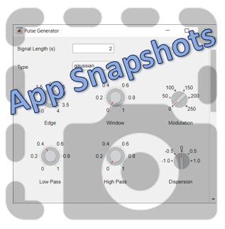
To demonstrate this, I adapted a copy of Matlab's built-in PulseGenerator.mlapp by adding

• a record button
• a record status lamp with frame counter
• a playback button
• a function that animates the effects of the Edge Knob

Recording process (The GIF is a lot faster than realtime and only shows part of the recording) (Open the image in a new window or see the attached Live Script for a clearer image).

Playback process (Open the image in a new window or see the attached Live Script for a clearer image.)

Review: How to get the handle to an app figure

To use either of these functions outside of app designer, you'll need to access the App's figure handle. By default, the HandleVisibility property of uifigures is set to off preventing the use of gcf to retrieve the figure handle. Here are 4 ways to access the app's figure handle from outside of the app.

1. Store the app's handle when opening the app.

app = myApp;
% Get the figure handle
figureHandle = app.myAppUIFigure;

2. Search for the figure handle using the app's name, tag, or any other unique property value

allfigs = findall(0, 'Type', 'figure'); % handle to all existing figures
figureHandle = findall(allfigs, 'Name', 'MyApp', 'Tag', 'MyUniqueTagName');

3. Change the HandleVisibility property to on or callback so that the figure handle is accessible by gcf anywhere or from within callback functions. This can be changed programmatically or from within the app designer component browser. Note, this is not recommended since any function that uses gcf such as axes(), clf(), etc can now access your app!.

4. If the app's figure handle is needed within a callback function external to the app, you could pass the app's figure handle in as an input variable or you could use gcbf() even if the HandleVisibility is off.

See a complete list of changes to the PulseGenerator app in the attached Live Script file to recreate the app.

Prior to r2020b the height (number of rows) and width (number of columns) of an array or table can be determined by the size function,

array = rand(102, 16);

% Method 1
[dimensions] = size(array);
h = dimensions(1);
w = dimensions(2);

% Method 2
[h, w] = size(array); %#ok<*ASGLU>
% or
[h, ~] = size(array);
[~, w] = size(array);

% Method 3
h = size(array,1);
w = size(array,2);

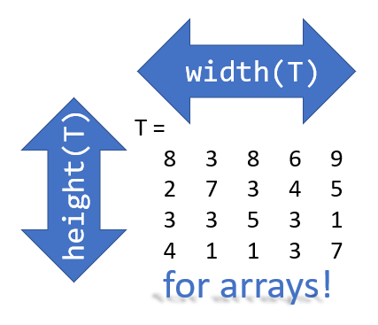
In r2013b, the height(T) and width(T) functions were introduced to return the size of single dimensions for tables and timetables.

Starting in r2020b, height() and width() can be applied to arrays as an alternative to the size() function.

Continuing from the section above,

h = height(array)
% h =  102

w = width(array)
% w =  16

height() and width() can also be applied to multidimensional arrays including cell and structure arrays

mdarray = rand(4,3,20);
h = height(mdarray)
% h =  4

w = width(mdarray)
% w =  3

The expanded support of the height() and width() functions means,

1. when reading code, you can no longer assume the variable T in height(T) or width(T) refers to a table or timetable
2. greater flexibility in expressions such as the these, below

% C is a 1x4 cell array containing 4 matrices with different dimensions
rng('default')
C = {rand(5,2), rand(2,3), rand(3,4), rand(1,1)};
celldisp(C)

% C{1} =
%       0.81472      0.09754
%       0.90579       0.2785
%       0.12699      0.54688
%       0.91338      0.95751
%       0.63236      0.96489
% C{2} =
%       0.15761      0.95717      0.80028
%       0.97059      0.48538      0.14189
% C{3} =
%       0.42176      0.95949      0.84913      0.75774
%       0.91574      0.65574      0.93399      0.74313
%       0.79221     0.035712      0.67874      0.39223
% C{4} =
%       0.65548

What's the max number of rows in C?

maxRows1 = max(cellfun(@height,C))         % using height()
% maxRows1 =  5;

maxRows2 = max(cellfun(@(x)size(x,1),C))   % using size()
% maxRows2 =  5; 

What's the total number of columns in C?

totCols1 = sum(cellfun(@width,C))          % using width()
%totCols1 =  10

totCols2 = sum(cellfun(@(x)size(x,2),C))   % using size(x,2)
% totCols2 =  10

Attached is a live script containing the content of this post.