Pull up a chair!
Discussions is your place to get to know your peers, tackle the bigger challenges together, and have fun along the way.
- Want to see the latest updates? Follow the Highlights!
- Looking for techniques improve your MATLAB or Simulink skills? Tips & Tricks has you covered!
- Sharing the perfect math joke, pun, or meme? Look no further than Fun!
- Think there's a channel we need? Tell us more in Ideas
Updated Discussions
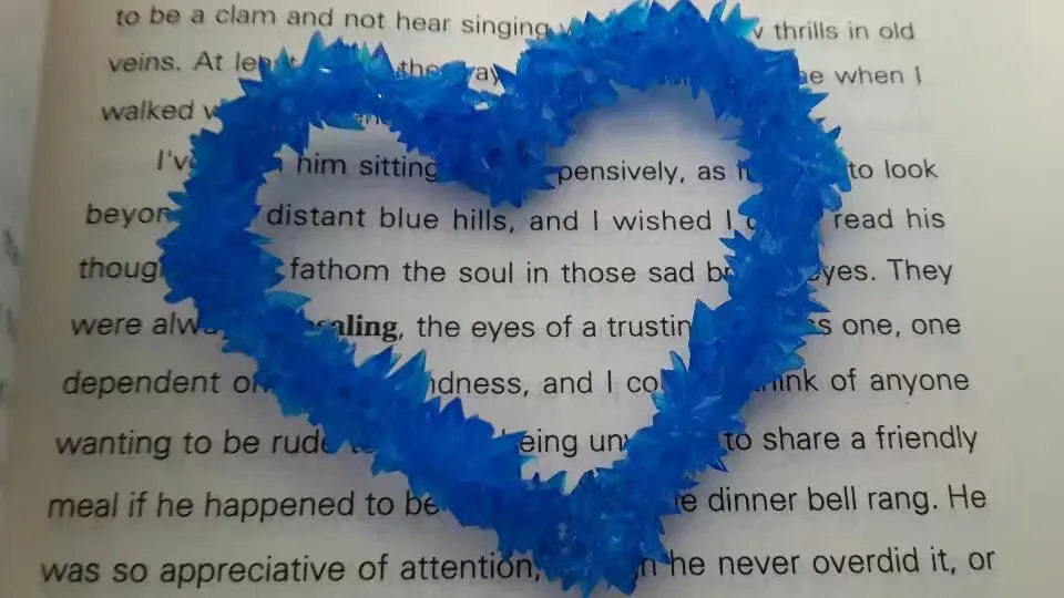
The creativity comes from the copper sulfate crystal heart made in junior high school. Copper sulfate is a triclinic crystal, and the same structure was not used here for convenience in drawing.
Part 1. Coordinate transformation
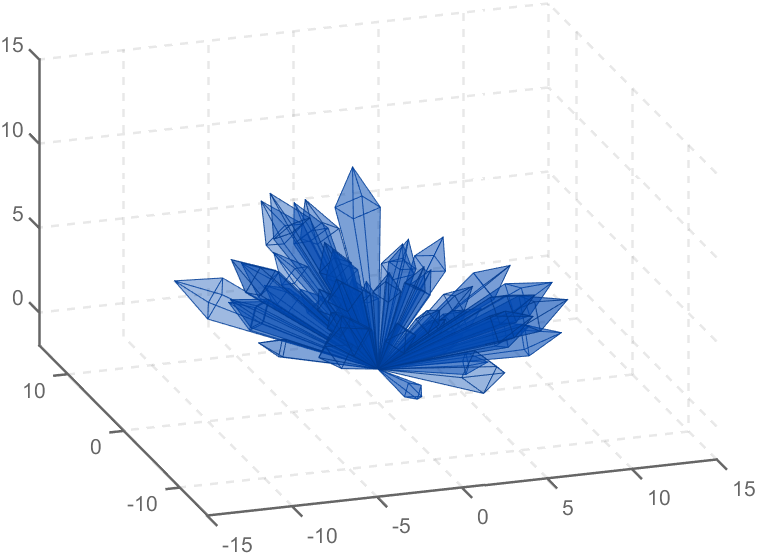
To draw a crystal heart, one must first be able to draw crystal clusters. To draw a crystal cluster, one must first be able to draw a crystal. To draw a crystal, we need this kind of structure:
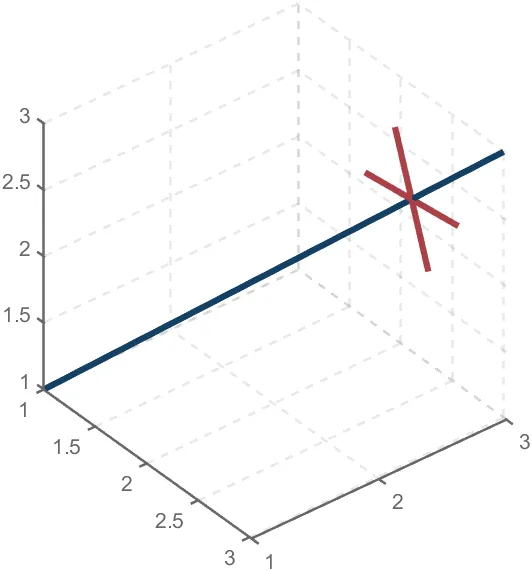
We first need a point with a certain distance from the straight line and a perpendicular point of cutPnt, which is very easy to find, for example, cutPnt=[x0, y0, z0]; The direction of the central axis is V=[x1, y1, z1]; If the distance to the straight line is L, the following points clearly meet the conditions:
v2=[z1,z1,-x1-y1];
v2=v2./norm(v2).*L;
pnt=cutPnt+v2;
But finding only one point is not enough. We need to find four points, and each point is obtained by rotating the previous point around a straight line by  degrees. Therefore, we need to obtain our point rotation transformation matrix around a straight line
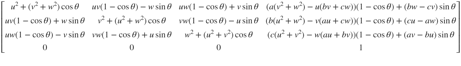
quite complex,right?
rotateMat=[u^2+(v^2+w^2)*cos(theta) , u*v*(1-cos(theta))-w*sin(theta), u*w*(1-cos(theta))+v*sin(theta), (a*(v^2+w^2)-u*(b*v+c*w))*(1-cos(theta))+(b*w-c*v)*sin(theta);
u*v*(1-cos(theta))+w*sin(theta), v^2+(u^2+w^2)*cos(theta) , v*w*(1-cos(theta))-u*sin(theta), (b*(u^2+w^2)-v*(a*u+c*w))*(1-cos(theta))+(c*u-a*w)*sin(theta);
u*w*(1-cos(theta))-v*sin(theta), v*w*(1-cos(theta))+u*sin(theta), w^2+(u^2+v^2)*cos(theta) , (c*(u^2+v^2)-w*(a*u+b*v))*(1-cos(theta))+(a*v-b*u)*sin(theta);
0 , 0 , 0 , 1];
Where [u, v, w] is the directional unit vector, and [a, b, c] is the initial coordinate of the axis:
Part 2. Crystal Cluster Drawing
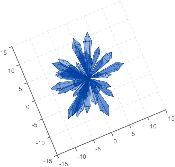
function crystall
hold on
for i=1:50
len=rand(1)*8+5;
tempV=rand(1,3)-0.5;
tempV(3)=abs(tempV(3));
tempV=tempV./norm(tempV).*len;
tempEpnt=tempV;
drawCrystal([0 0 0],tempEpnt,pi/6,0.8,0.1,rand(1).*0.2+0.2)
disp(i)
end
ax=gca;
ax.XLim=[-15,15];
ax.YLim=[-15,15];
ax.ZLim=[-2,15];
grid on
ax.GridLineStyle='--';
ax.LineWidth=1.2;
ax.XColor=[1,1,1].*0.4;
ax.YColor=[1,1,1].*0.4;
ax.ZColor=[1,1,1].*0.4;
ax.DataAspectRatio=[1,1,1];
ax.DataAspectRatioMode='manual';
ax.CameraPosition=[-67.6287 -204.5276 82.7879];
function drawCrystal(Spnt,Epnt,theta,cl,w,alpha)
%plot3([Spnt(1),Epnt(1)],[Spnt(2),Epnt(2)],[Spnt(3),Epnt(3)])
mainV=Epnt-Spnt;
cutPnt=cl.*(mainV)+Spnt;
cutV=[mainV(3),mainV(3),-mainV(1)-mainV(2)];
cutV=cutV./norm(cutV).*w.*norm(mainV);
cornerPnt=cutPnt+cutV;
cornerPnt=rotateAxis(Spnt,Epnt,cornerPnt,theta);
cornerPntSet(1,:)=cornerPnt';
for ii=1:3
cornerPnt=rotateAxis(Spnt,Epnt,cornerPnt,pi/2);
cornerPntSet(ii+1,:)=cornerPnt';
end
F = [1,3,4;1,4,5;1,5,6;1,6,3;...
2,3,4;2,4,5;2,5,6;2,6,3];
V = [Spnt;Epnt;cornerPntSet];
patch('Faces',F,'Vertices',V,'FaceColor',[0 71 177]./255,...
'FaceAlpha',alpha,'EdgeColor',[0 71 177]./255.*0.8,...
'EdgeAlpha',0.6,'LineWidth',0.5,'EdgeLighting',...
'gouraud','SpecularStrength',0.3)
end
function newPnt=rotateAxis(Spnt,Epnt,cornerPnt,theta)
V=Epnt-Spnt;V=V./norm(V);
u=V(1);v=V(2);w=V(3);
a=Spnt(1);b=Spnt(2);c=Spnt(3);
cornerPnt=[cornerPnt(:);1];
rotateMat=[u^2+(v^2+w^2)*cos(theta) , u*v*(1-cos(theta))-w*sin(theta), u*w*(1-cos(theta))+v*sin(theta), (a*(v^2+w^2)-u*(b*v+c*w))*(1-cos(theta))+(b*w-c*v)*sin(theta);
u*v*(1-cos(theta))+w*sin(theta), v^2+(u^2+w^2)*cos(theta) , v*w*(1-cos(theta))-u*sin(theta), (b*(u^2+w^2)-v*(a*u+c*w))*(1-cos(theta))+(c*u-a*w)*sin(theta);
u*w*(1-cos(theta))-v*sin(theta), v*w*(1-cos(theta))+u*sin(theta), w^2+(u^2+v^2)*cos(theta) , (c*(u^2+v^2)-w*(a*u+b*v))*(1-cos(theta))+(a*v-b*u)*sin(theta);
0 , 0 , 0 , 1];
newPnt=rotateMat*cornerPnt;
newPnt(4)=[];
end
end
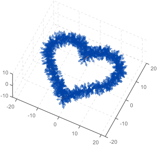
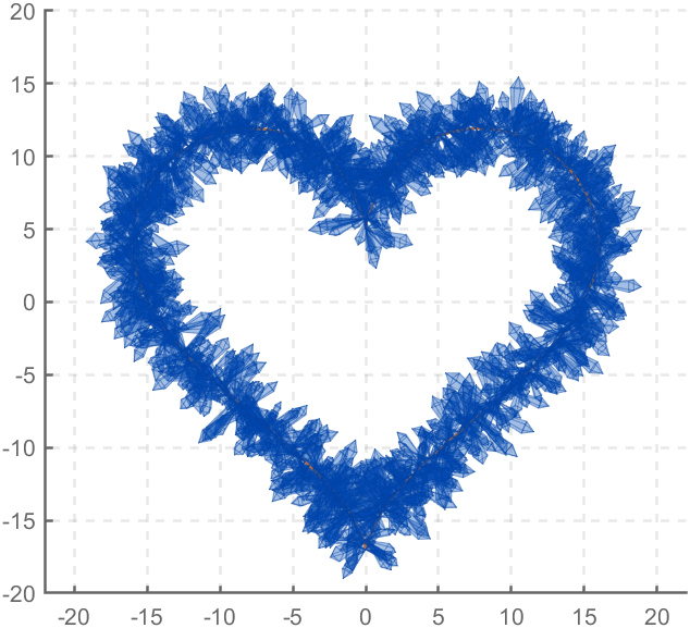
Part 3. Drawing of Crystal Heart
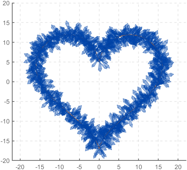
function crystalHeart
clc;clear;close all
hold on
% drawCrystal([1,1,1],[3,3,3],pi/6,0.8,0.14)
sep=pi/8;
t=[0:0.2:sep,sep:0.02:pi-sep,pi-sep:0.2:pi+sep,pi+sep:0.02:2*pi-sep,2*pi-sep:0.2:2*pi];
x=16*sin(t).^3;
y=13*cos(t)-5*cos(2*t)-2*cos(3*t)-cos(4*t);
z=zeros(size(t));
plot3(x,y,z,'Color',[186,110,64]./255,'LineWidth',1)
for i=1:length(t)
for j=1:6
len=rand(1)*2.5+1.5;
tempV=rand(1,3)-0.5;
tempV=tempV./norm(tempV).*len;
tempSpnt=[x(i),y(i),z(i)];
tempEpnt=tempV+tempSpnt;
drawCrystal(tempSpnt,tempEpnt,pi/6,0.8,0.14)
disp([i,j])
end
end
ax=gca;
ax.XLim=[-22,22];
ax.YLim=[-20,20];
ax.ZLim=[-10,10];
grid on
ax.GridLineStyle='--';
ax.LineWidth=1.2;
ax.XColor=[1,1,1].*0.4;
ax.YColor=[1,1,1].*0.4;
ax.ZColor=[1,1,1].*0.4;
ax.DataAspectRatio=[1,1,1];
ax.DataAspectRatioMode='manual';
function drawCrystal(Spnt,Epnt,theta,cl,w)
%plot3([Spnt(1),Epnt(1)],[Spnt(2),Epnt(2)],[Spnt(3),Epnt(3)])
mainV=Epnt-Spnt;
cutPnt=cl.*(mainV)+Spnt;
cutV=[mainV(3),mainV(3),-mainV(1)-mainV(2)];
cutV=cutV./norm(cutV).*w.*norm(mainV);
cornerPnt=cutPnt+cutV;
cornerPnt=rotateAxis(Spnt,Epnt,cornerPnt,theta);
cornerPntSet(1,:)=cornerPnt';
for ii=1:3
cornerPnt=rotateAxis(Spnt,Epnt,cornerPnt,pi/2);
cornerPntSet(ii+1,:)=cornerPnt';
end
F = [1,3,4;1,4,5;1,5,6;1,6,3;...
2,3,4;2,4,5;2,5,6;2,6,3];
V = [Spnt;Epnt;cornerPntSet];
patch('Faces',F,'Vertices',V,'FaceColor',[0 71 177]./255,...
'FaceAlpha',0.2,'EdgeColor',[0 71 177]./255.*0.9,...
'EdgeAlpha',0.25,'LineWidth',0.01,'EdgeLighting',...
'gouraud','SpecularStrength',0.3)
end
function newPnt=rotateAxis(Spnt,Epnt,cornerPnt,theta)
V=Epnt-Spnt;V=V./norm(V);
u=V(1);v=V(2);w=V(3);
a=Spnt(1);b=Spnt(2);c=Spnt(3);
cornerPnt=[cornerPnt(:);1];
rotateMat=[u^2+(v^2+w^2)*cos(theta) , u*v*(1-cos(theta))-w*sin(theta), u*w*(1-cos(theta))+v*sin(theta), (a*(v^2+w^2)-u*(b*v+c*w))*(1-cos(theta))+(b*w-c*v)*sin(theta);
u*v*(1-cos(theta))+w*sin(theta), v^2+(u^2+w^2)*cos(theta) , v*w*(1-cos(theta))-u*sin(theta), (b*(u^2+w^2)-v*(a*u+c*w))*(1-cos(theta))+(c*u-a*w)*sin(theta);
u*w*(1-cos(theta))-v*sin(theta), v*w*(1-cos(theta))+u*sin(theta), w^2+(u^2+v^2)*cos(theta) , (c*(u^2+v^2)-w*(a*u+b*v))*(1-cos(theta))+(a*v-b*u)*sin(theta);
0 , 0 , 0 , 1];
newPnt=rotateMat*cornerPnt;
newPnt(4)=[];
end
end
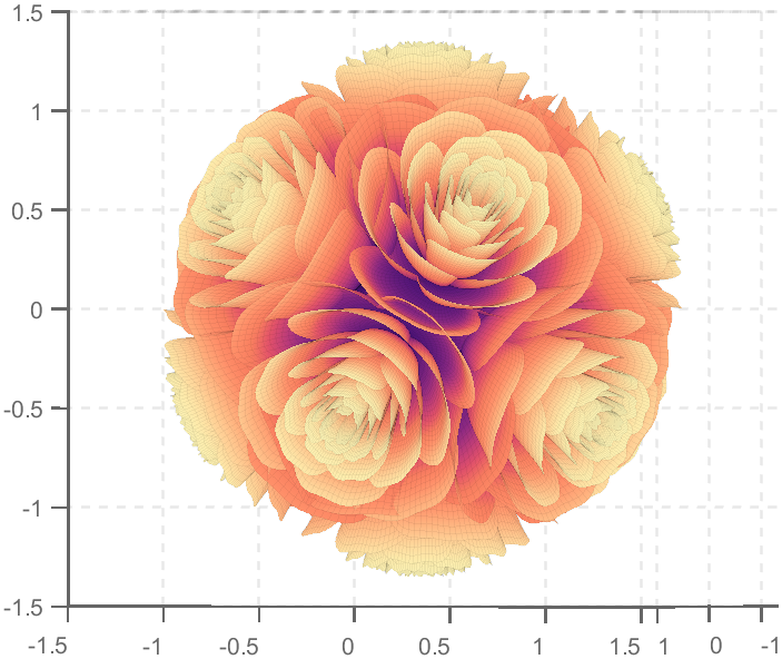
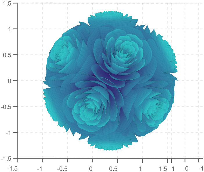
So, how to draw a roseball just like this ?
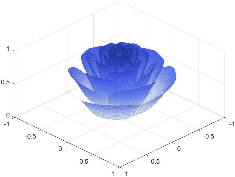
To begin with, we need to know how to draw a single rose in MATLAB:
function drawrose
set(gca,'CameraPosition',[2 2 2])
hold on
grid on
[x,t]=meshgrid((0:24)./24,(0:0.5:575)./575.*20.*pi+4*pi);
p=(pi/2)*exp(-t./(8*pi));
change=sin(15*t)/150;
u=1-(1-mod(3.6*t,2*pi)./pi).^4./2+change;
y=2*(x.^2-x).^2.*sin(p);
r=u.*(x.*sin(p)+y.*cos(p));
h=u.*(x.*cos(p)-y.*sin(p));
surface(r.*cos(t),r.*sin(t),h,'EdgeAlpha',0.1,...
'EdgeColor',[0 0 0],'FaceColor','interp')
end
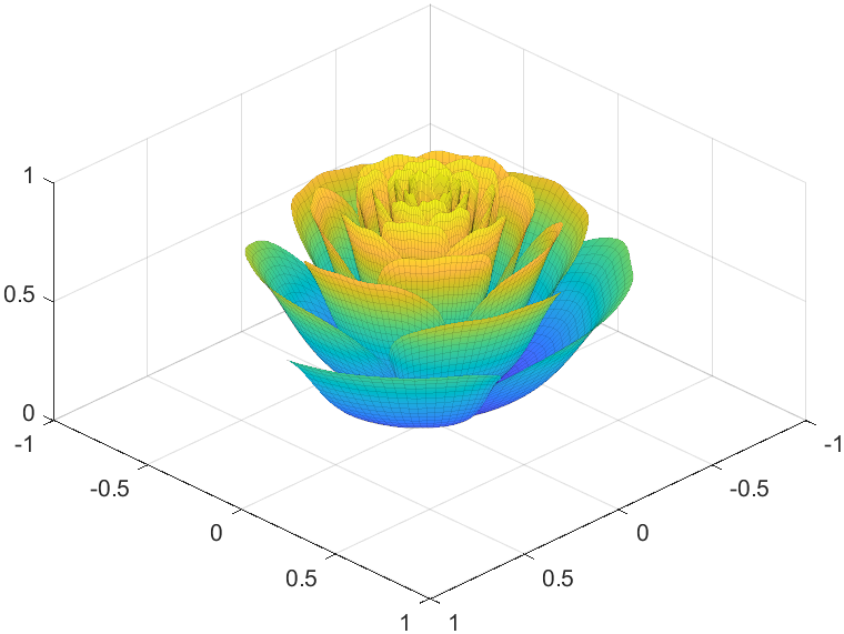
Tts pretty easy, Now we are trying to dye it the desired color:
function drawrose
set(gca,'CameraPosition',[2 2 2])
hold on
grid on
[x,t]=meshgrid((0:24)./24,(0:0.5:575)./575.*20.*pi+4*pi);
p=(pi/2)*exp(-t./(8*pi));
change=sin(15*t)/150;
u=1-(1-mod(3.6*t,2*pi)./pi).^4./2+change;
y=2*(x.^2-x).^2.*sin(p);
r=u.*(x.*sin(p)+y.*cos(p));
h=u.*(x.*cos(p)-y.*sin(p));
map=[0.9176 0.9412 1.0000
0.8353 0.8706 0.9922
0.8196 0.8627 0.9804
0.7020 0.7569 0.9412
0.5176 0.5882 0.9255
0.3686 0.4824 0.9412
0.3059 0.4000 0.9333
0.2275 0.3176 0.8353
0.1216 0.2275 0.6471];
Xi=1:size(map,1);Xq=linspace(1,size(map,1),100);
map=[interp1(Xi,map(:,1),Xq,'linear')',...
interp1(Xi,map(:,2),Xq,'linear')',...
interp1(Xi,map(:,3),Xq,'linear')'];
surface(r.*cos(t),r.*sin(t),h,'EdgeAlpha',0.1,...
'EdgeColor',[0 0 0],'FaceColor','interp')
colormap(map)
end
I try to take colors from real roses and interpolate them to make them more realistic
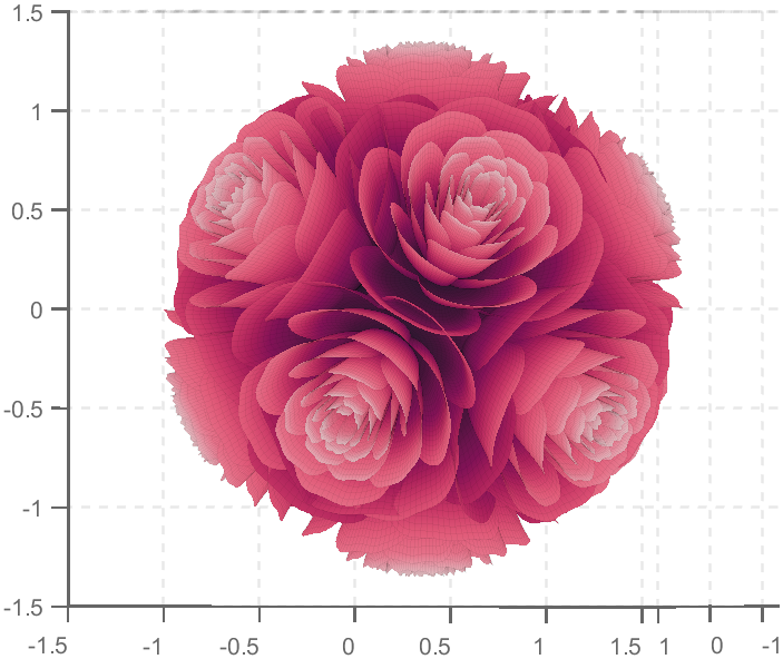
Then, how can I put these colorful flowers on to a ball ?
We need to place the drawn flowers on each face of the polyhedron sphere through coordinate transformation. Here, we use a regular dodecahedron:
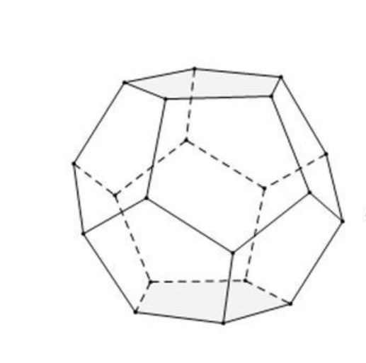
Move the flower using the following rotation formula:
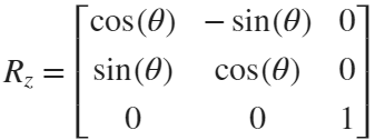
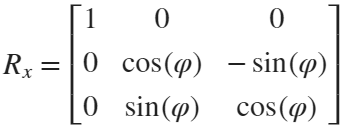
We place a flower on each plane, which means that the angle between every two flowers is 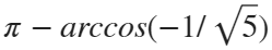 degrees. We can place each flower at the appropriate angle through multiple x-axis rotations and multiple z-axis rotations. The code is as follows:
function roseBall(colorList)
%曲面数据计算
%==========================================================================
[x,t]=meshgrid((0:24)./24,(0:0.5:575)./575.*20.*pi+4*pi);
p=(pi/2)*exp(-t./(8*pi));
change=sin(15*t)/150;
u=1-(1-mod(3.6*t,2*pi)./pi).^4./2+change;
y=2*(x.^2-x).^2.*sin(p);
r=u.*(x.*sin(p)+y.*cos(p));
h=u.*(x.*cos(p)-y.*sin(p));
%颜色映射表
%==========================================================================
hMap=(h-min(min(h)))./(max(max(h))-min(min(h)));
col=size(hMap,2);
if nargin<1
colorList=[0.0200 0.0400 0.3900
0 0.0900 0.5800
0 0.1300 0.6400
0.0200 0.0600 0.6900
0 0.0800 0.7900
0.0100 0.1800 0.8500
0 0.1300 0.9600
0.0100 0.2600 0.9900
0 0.3500 0.9900
0.0700 0.6200 1.0000
0.1700 0.6900 1.0000];
end
colorFunc=colorFuncFactory(colorList);
dataMap=colorFunc(hMap');
colorMap(:,:,1)=dataMap(:,1:col);
colorMap(:,:,2)=dataMap(:,col+1:2*col);
colorMap(:,:,3)=dataMap(:,2*col+1:3*col);
function colorFunc=colorFuncFactory(colorList)
xx=(0:size(colorList,1)-1)./(size(colorList,1)-1);
y1=colorList(:,1);y2=colorList(:,2);y3=colorList(:,3);
colorFunc=@(X)[interp1(xx,y1,X,'linear')',interp1(xx,y2,X,'linear')',interp1(xx,y3,X,'linear')'];
end
%曲面旋转及绘制
%==========================================================================
surface(r.*cos(t),r.*sin(t),h+0.35,'EdgeAlpha',0.05,...
'EdgeColor',[0 0 0],'FaceColor','interp','CData',colorMap)
hold on
surface(r.*cos(t),r.*sin(t),-h-0.35,'EdgeAlpha',0.05,...
'EdgeColor',[0 0 0],'FaceColor','interp','CData',colorMap)
Xset=r.*cos(t);
Yset=r.*sin(t);
Zset=h+0.35;
yaw_z=72*pi/180;
roll_x=pi-acos(-1/sqrt(5));
R_z_2=[cos(yaw_z),-sin(yaw_z),0;
sin(yaw_z),cos(yaw_z),0;
0,0,1];
R_z_1=[cos(yaw_z/2),-sin(yaw_z/2),0;
sin(yaw_z/2),cos(yaw_z/2),0;
0,0,1];
R_x_2=[1,0,0;
0,cos(roll_x),-sin(roll_x);
0,sin(roll_x),cos(roll_x)];
[nX,nY,nZ]=rotateXYZ(Xset,Yset,Zset,R_x_2);
surface(nX,nY,nZ,'EdgeAlpha',0.05,...
'EdgeColor',[0 0 0],'FaceColor','interp','CData',colorMap)
for k=1:4
[nX,nY,nZ]=rotateXYZ(nX,nY,nZ,R_z_2);
surface(nX,nY,nZ,'EdgeAlpha',0.05,...
'EdgeColor',[0 0 0],'FaceColor','interp','CData',colorMap)
end
[nX,nY,nZ]=rotateXYZ(nX,nY,nZ,R_z_1);
for k=1:5
[nX,nY,nZ]=rotateXYZ(nX,nY,nZ,R_z_2);
surface(nX,nY,-nZ,'EdgeAlpha',0.05,...
'EdgeColor',[0 0 0],'FaceColor','interp','CData',colorMap)
end
%--------------------------------------------------------------------------
function [nX,nY,nZ]=rotateXYZ(X,Y,Z,R)
nX=zeros(size(X));
nY=zeros(size(Y));
nZ=zeros(size(Z));
for i=1:size(X,1)
for j=1:size(X,2)
v=[X(i,j);Y(i,j);Z(i,j)];
nv=R*v;
nX(i,j)=nv(1);
nY(i,j)=nv(2);
nZ(i,j)=nv(3);
end
end
end
%axes属性调整
%==========================================================================
ax=gca;
grid on
ax.GridLineStyle='--';
ax.LineWidth=1.2;
ax.XColor=[1,1,1].*0.4;
ax.YColor=[1,1,1].*0.4;
ax.ZColor=[1,1,1].*0.4;
ax.DataAspectRatio=[1,1,1];
ax.DataAspectRatioMode='manual';
ax.CameraPosition=[-6.5914 -24.1625 -0.0384];
end

TRY DIFFERENT COLORS !!
colorList1=[0.2000 0.0800 0.4300
0.2000 0.1300 0.4600
0.2000 0.2100 0.5000
0.2000 0.2800 0.5300
0.2000 0.3700 0.5800
0.1900 0.4500 0.6200
0.2000 0.4800 0.6400
0.1900 0.5400 0.6700
0.1900 0.5700 0.6900
0.1900 0.7500 0.7800
0.1900 0.8000 0.8100
];
colorList2=[0.1300 0.1000 0.1600
0.2000 0.0900 0.2000
0.2800 0.0800 0.2300
0.4200 0.0800 0.3000
0.5100 0.0700 0.3400
0.6600 0.1200 0.3500
0.7900 0.2200 0.4000
0.8800 0.3500 0.4700
0.9000 0.4500 0.5400
0.8900 0.7800 0.7900
];
colorList3=[0.3200 0.3100 0.7600
0.3800 0.3400 0.7600
0.5300 0.4200 0.7500
0.6400 0.4900 0.7300
0.7200 0.5500 0.7200
0.7900 0.6100 0.7100
0.9100 0.7100 0.6800
0.9800 0.7600 0.6700
];
colorList4=[0.2100 0.0900 0.3800
0.2900 0.0700 0.4700
0.4000 0.1100 0.4900
0.5500 0.1600 0.5100
0.7500 0.2400 0.4700
0.8900 0.3200 0.4100
0.9700 0.4900 0.3700
1.0000 0.5600 0.4100
1.0000 0.6900 0.4900
1.0000 0.8200 0.5900
0.9900 0.9200 0.6700
0.9800 0.9500 0.7100];
Can anyone provide insight into the intended difference between Discussions and Answers and what should be posted where?
Just scrolling through Discussions, I saw postst that seem more suitable Answers?
What exactly does Discussions bring to the table that wasn't already brought by Answers?
Maybe this question is more suitable for a Discussion ....
Would it be a good thing to have implicit expansion enabled for cat(), horzcat(), vertcat()? There are often situations where I would like to be able to do things like this:
x=[10;20;30;40];
y=[11;12;13;14];
z=cat(3, 0,1,2);
C=[x,y,z]
with the result,
C(:,:,1) =
10 11 0
20 12 0
30 13 0
40 14 0
C(:,:,2) =
10 11 1
20 12 1
30 13 1
40 14 1
C(:,:,3) =
10 11 2
20 12 2
30 13 2
40 14 2
Let us consider how to draw a Happy Sheep. A Happy Sheep was introduced in the MATLAB Mini Hack contest: Happy Sheep!
In this contest there was the strict limitation on the code length. So the code of the Happy Sheep is very compact and is only 280 characters long. We will analyze the process of drawing the Happy Sheep in MATLAB step by step. The explanations of the even more compact version of the code of the same sheep are given below.
So, how to draw a sheep? It is very easy. We could notice that usually a sheep is covered by crimped wool. Therefore, a sheep could be painted using several geometrical curves of similar types. Of course, then it will be an abstract model of the real sheep. Let us select two mathematical curves, which are the most appropriate for our goal. They are an ellipse for smooth parts of the sheep and an ellipse combined with a rose for woolen parts of the sheep.
Let us recall the mathematical formulas of these curves. A parametric representation of the standard ellipse is the following:
Also we will use the following parametric representation of the rose (rhodonea) curve:
This curve was named by the mathematician Guido Grandi.
Let us combine them in one curve and add possible shifts:
Now if we would like to create an ellipse, we will set  and
and  . If we would like to create a rose, we will set
  and
and  . If we would like to shift our curve, we will set
  and
and  to the required values. Of course, we could set all non-zero parameters to combine both chosen curves and use the shifts.
Let us describe how to create these curves using the MATLAB code. To make the code more compact, it is possible to program both formulas for the combined curve in one line using the anonymous function. We could make the code more compact using the function handles for sine and cosine functions. Then the MATLAB code for an example of the ellipse curve will be the following.
% Handles
s=@sin;
c=@cos;
% Ellipse + Polar Rose
F=@(t,a,f) a(1)*f(t)+s(a(2)*t).*f(t)+a(3);
% Angles
t=0:.1:7;
% Parameters
E = [5 7;0 0;0 0];
% Painting
figure;
plot(F(t,E(:,1),c),F(t,E(:,2),s),'LineWidth',10);
axis equal
The parameter t varies from 0 to 7, which is the nearest integer greater than  , with the step 0.1. The result of this code is the following ellipse curve with
  and
and  .
.
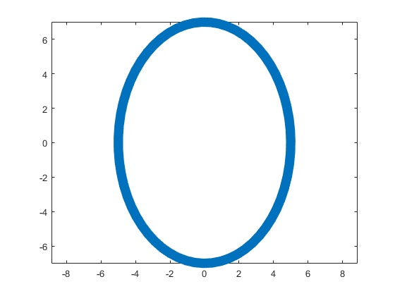
This ellipse is described by the following parametric equations:
The MATLAB code for an example of the rose curve will be the following.
% Handles
s=@sin;
c=@cos;
% Ellipse + Polar Rose
F=@(t,a,f) a(1)*f(t)+s(a(2)*t).*f(t)+a(3);
% Angles
t=0:.1:7;
% Parameters
R = [0 0;4 4;0 0];
% Painting
figure;
plot(F(t,R(:,1),c),F(t,R(:,2),s),'LineWidth',10);
axis equal
The result of this code is the following rose curve with  and
and  .
.
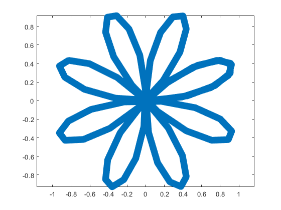
This rose is described by the following parametric equations:
Obviously, now we are ready to draw main parts of our sheep! As we reproduce an abstract model of the sheep, let us select the following main parts for the representation: head, eyes, hoofs, body, crown, and tail. We will use ellipses for the first three parts in this list and ellipses combined with roses for the last three ones.
First let us describe drawing of each part independently.
The following MATLAB code will be used to do this.
% Handles
s=@sin;
c=@cos;
% Ellipse + Polar Rose
F=@(t,a,f) a(1)*f(t)+s(a(2)*t).*f(t)+a(3);
% Angles
t=0:.1:7;
% Parameters
Head = 1;
Eyes = 2:3;
Hoofs = 4:7;
Body = 8;
Crown = 9;
Tail = 10;
G=-13;
P=[5 7 repmat([.1 .5],1,6) 6 4 14 9 3 3;zeros(1,14) 8 8 12 12 4 4;...
-15 2 G 3 -17 3 -3 G 0 G 9 G 12 G -15 12 4 3 20 7];
% Painting
figure;
hold;
for i=Head
plot(F(t,P(:,2*i-1),c),F(t,P(:,2*i),s),'LineWidth',10);
end
axis([-25 25 -15 20]);
figure;
hold;
for i=Eyes
plot(F(t,P(:,2*i-1),c),F(t,P(:,2*i),s),'LineWidth',10);
end
axis([-25 25 -15 20]);
figure;
hold;
for i=Hoofs
plot(F(t,P(:,2*i-1),c),F(t,P(:,2*i),s),'LineWidth',10);
end
axis([-25 25 -15 20]);
figure;
hold;
for i=Body
plot(F(t,P(:,2*i-1),c),F(t,P(:,2*i),s),'LineWidth',10);
end
axis([-25 25 -15 20]);
figure;
hold;
for i=Crown
plot(F(t,P(:,2*i-1),c),F(t,P(:,2*i),s),'LineWidth',10);
end
axis([-25 25 -15 20]);
figure;
hold;
for i=Tail
plot(F(t,P(:,2*i-1),c),F(t,P(:,2*i),s),'LineWidth',10);
end
axis([-25 25 -15 20]);
The parameters  ,
,  ,
,  ,
,  ,
,  , and
, and  are written in the different submatrices of the matrix P. The code generates the following curves to illustrate the different parts of our sheep.
The following ellipse describes the head of the sheep.
The following submatrix of the matrix P represents its parameters.
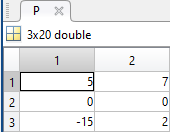
The parametric equations of the head are the following:
The following ellipses describe the eyes of the sheep.
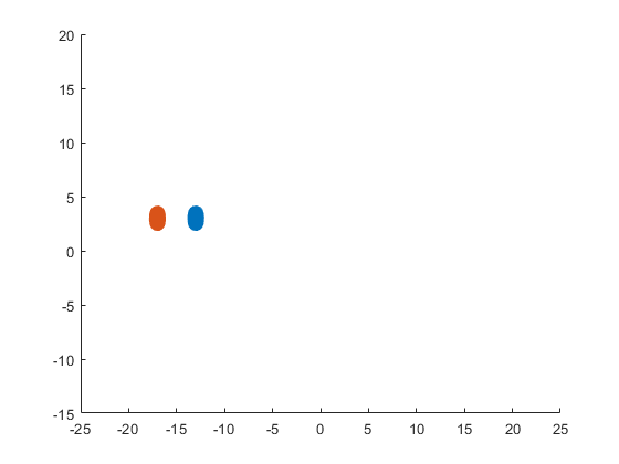
The following submatrices of the matrix P represent their parameters.
The parametric equations of the left and right eyes correspondingly are the following:
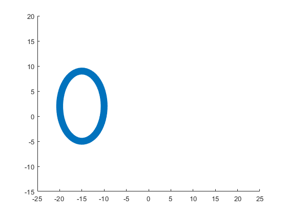
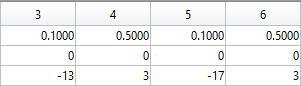
The following ellipses describe the hoofs of the sheep.
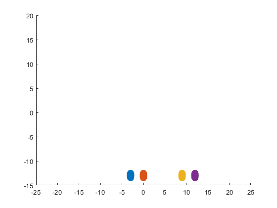
The following submatrices of the matrix P represent their parameters.
The parametric equations of the right front, left front, right hind, and left hind hoofs correspondingly are the following:
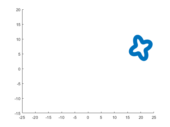
The following ellipse combined with the rose describes the crown of the sheep.
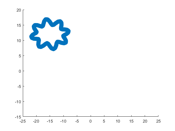
The following submatrix of the matrix P represents its parameters.
The parametric equations of the crown are the following:
The following ellipse combined with the rose describes the body of the sheep.
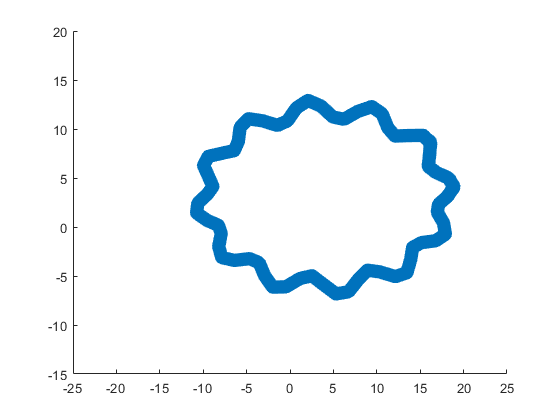
The following submatrix of the matrix P represents its parameters.
The parametric equations of the body are the following:
The following ellipse combined with the rose describes the tail of the sheep.
The following submatrix of the matrix P represents its parameters.
The parametric equations of the tail are the following:
Now all the parts of our sheep should be put together! It is very easy because all the parts are described by the same equations with different parameters.
The following code helps us to accomplish this goal and ultimately draw a Happy Sheep in MATLAB!
% Happy Sheep!
% By Victoria A. Sablina
% Handles
s=@sin;
c=@cos;
% Ellipse + Rose
F=@(t,a,f) a(1)*f(t)+s(a(2)*t).*f(t)+a(3);
% Angles
t=0:.1:7;
% Parameters
% Head (1:2)
% Eyes (3:6)
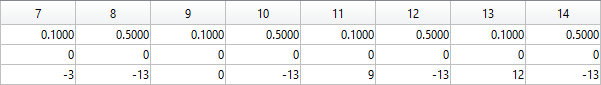
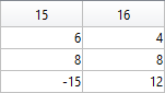
% Hoofs (7:14)
% Crown (15:16)
% Body (17:18)
% Tail (19:20)
G=-13;
P=[5 7 repmat([.1 .5],1,6) 6 4 14 9 3 3;zeros(1,14) 8 8 12 12 4 4;...
-15 2 G 3 -17 3 -3 G 0 G 9 G 12 G -15 12 4 3 20 7];
% Painting
hold;
for i=1:10
plot(F(t,P(:,2*i-1),c),F(t,P(:,2*i),s),'LineWidth',10);
end
This code is even more compact than the original code from the contest. It is only 253 instead of 280 characters long and generates the same Happy Sheep!
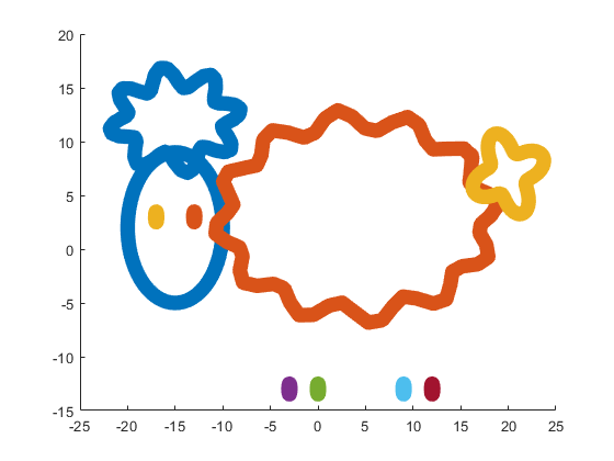
Our sheep is happy, because of becoming famous in the MATLAB community, a star!
Congratulations! Now you know how to draw a Happy Sheep in MATLAB!
Thank you for reading!
To enlarge an array with more rows and/or columns, you can set the lower right index to zero. This will pad the matrix with zeros.
m = rand(2, 3) % Initial matrix is 2 rows by 3 columns
mCopy = m;
% Now make it 2 rows by 5 columns
m(2, 5) = 0
m = mCopy; % Go back to original matrix.
% Now make it 3 rows by 3 columns
m(3, 3) = 0
m = mCopy; % Go back to original matrix.
% Now make it 3 rows by 7 columns
m(3, 7) = 0
how to generate CA signed certificate for mqtt
Due to temporary problem MathWorks account was unable to login. Kindly resolve this issue.
I asked my question in the general forum and a few minutes later it was deleted. Perhaps this is a better place?
Rather than using my German regional forum (as I do not speak German), I want to ask questions in an international English-speaking forum. Presumably there should be an international English forum for everyone around the world, as English is the first or second language of everyone who has gone to school. Where is it?
Big congratulations to @VBBV for achieving the remarkable milestone of 3,000 reputation points, earning the prestigious title of Editor within our community.
This achievement is a testament to @VBBV's exceptional contributions and steadfast commitment to the community. These efforts have also been endorsed by fellow top contributors, underscoring the value and impact of @VBBV's expertise.
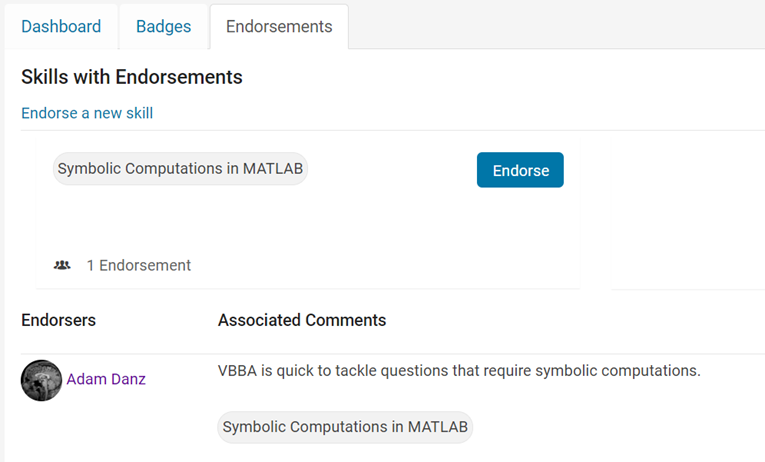
Welcome to the Editors' Club, @VBBV – we are excited to witness and support your continued journey and influence within our community!
MATLAB O/X Quiz
Answer BEFORE Googling!
- An infinite loop can be made using "for".
- "A == A" is always true.
- "round(2.5)" is 3.
- "round(-0.5)" is 0.
How do I can delete my account?
We have to create a few 10s of channels all with the same public view and settings. Is there any way of automating this ?
Doing it manually is time consuming and results in omissions and small mistakes.
When I embed Matlab windows into C#, I use C# to call the mouse functions such as drawline() and getpts() which are encapsulated in Matlab's dll, and then the program crashes, how can I solve this problem?
ps : The functions that I call in C# can be executed in Matlab.
ps : If I don't embed the window into C#, but just let C# call the Matlab function, it can execute the mouse control normally in the window, but once embedded into the C# window, it will crash when execute the mouse command.
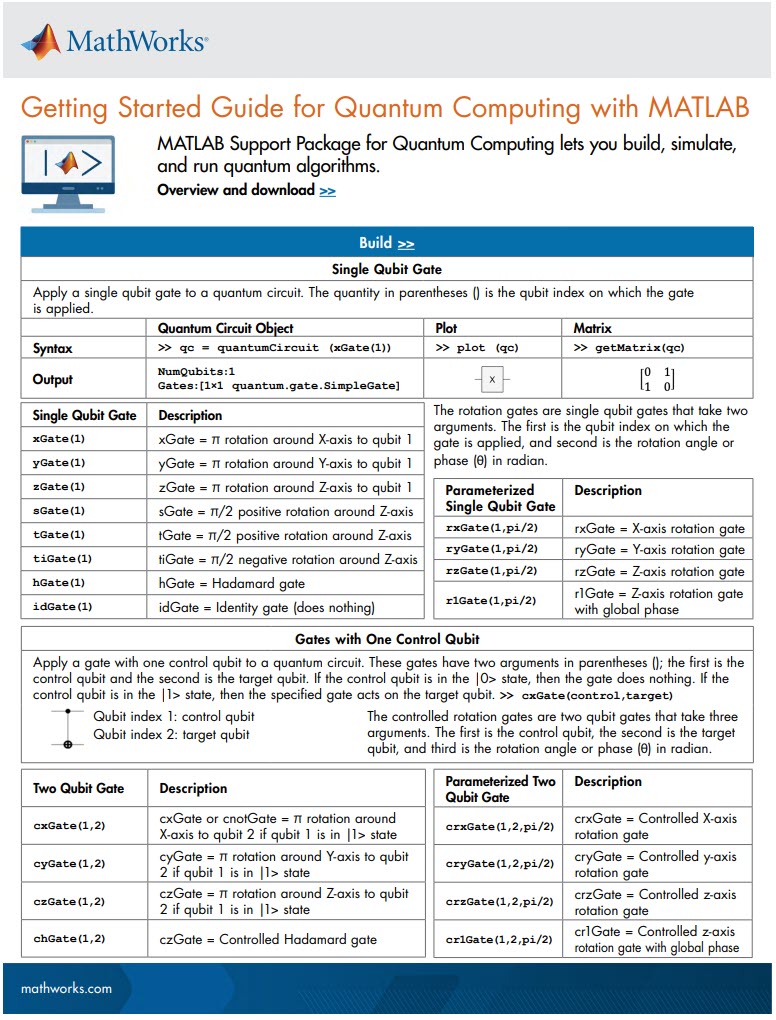
MATLAB Support Package for Quantum Computing lets you build, simulate, and run quantum algorithms.
Check out the Cheat Sheet here!
I am confused, is the matlab answer better or Julia’s?
2 x 2 행렬의 행렬식은
- 행렬의 두 row 벡터로 정의되는 평행사변형의 면적입니다.
- 물론 두 column 벡터로 정의되는 평행사변형의 면적이기도 합니다.
- 좀 더 정확히는 signed area입니다. 면적이 음수가 될 수도 있다는 뜻이죠.
- 행렬의 두 행(또는 두 열)을 맞바꾸면 행렬식의 부호도 바뀌고 면적의 부호도 바뀌어야합니다.
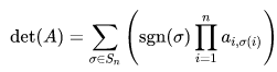
일반적으로 n x n 행렬의 행렬식은
- 각 row 벡터(또는 각 column 벡터)로 정의되는 N차원 공간의 평행면체(?)의 signed area입니다.
- 제대로 이해하려면 대수학의 개념을 많이 가지고 와야 하는데 자세한 설명은 생략합니다.(=저도 모른다는 뜻)
- 더 자세히 알고 싶으시면 수학하는 만화의 '넓이 이야기' 편을 추천합니다.
- 수학적인 정의를 알고 싶으시면 위키피디아를 보시면 됩니다.
- 이렇게 생겼습니다. 좀 무섭습니다.
아래 코드는...
- 2 x 2 행렬에 대해서 이것을 수식 없이 그림만으로 증명하는 과정입니다.
- gif 생성에는 ScreenToGif를 사용했습니다. (gif 만들기엔 이게 킹왕짱인듯)
Determinant of 2 x 2 matrix is...
- An area of a parallelogram defined by two row vectors.
- Of course, same one defined by two column vectors.
- Precisely, a signed area, which means area can be negative.
- If two rows (or columns) are swapped, both the sign of determinant and area change.
More generally, determinant of n x n matrix is...
- Signed area of parallelepiped defined by rows (or columns) of the matrix in n-dim space.
- For a full understanding, a lot of concepts from abstract algebra should be brought, which I will not write here. (Cuz I don't know them.)
- For a mathematical definition of determinant, visit wikipedia.

- A little scary, isn't it?
The code below is...
- A process to prove the equality of the determinant of 2 x 2 matrix and the area of parallelogram.
- ScreenToGif is used to generate gif animation (which is, to me, the easiest way to make gif).
% 두 점 (a, b), (c, d)의 좌표
a = 4;
b = 1;
c = 1;
d = 3;
% patch 색 pre-define
lightgreen = [144, 238, 144]/255;
lightblue = [169, 190, 228]/255;
lightorange = [247, 195, 160]/255;
% animation params.
anim_Nsteps = 30;
% create window
figure('WindowStyle','docked')
ax = axes;
ax.XAxisLocation = 'origin';
ax.YAxisLocation = 'origin';
ax.XTick = [];
ax.YTick = [];
hold on
ax.XLim = [-.4, a+c+1];
ax.YLim = [-.4, b+d+1];
% create ad-bc patch
area = patch([0, a, a+c, c], [0, b, b+d, d], lightgreen);
p_ab = plot(a, b, 'ko', 'MarkerFaceColor', 'k');
p_cd = plot(c, d, 'ko', 'MarkerFaceColor', 'k');
p_ab.UserData = text(a+0.1, b, '(a, b)', 'FontSize',16);
p_cd.UserData = text(c+0.1, d-0.2, '(c, d)', 'FontSize',16);
area.UserData = text((a+c)/2-0.5, (b+d)/2, 'ad-bc', 'FontSize', 18);
pause
%% Is this really ad-bc?
area.UserData.String = 'ad-bc...?';
pause
%% fade out ad-bc
fadeinout(area, 0)
area.UserData.Visible = 'off';
pause
%% fade in ad block
rect_ad = patch([0, a, a, 0], [0, 0, d, d], lightblue, 'EdgeAlpha', 0, 'FaceAlpha', 0);
uistack(rect_ad, 'bottom');
fadeinout(rect_ad, 1, t_pause=0.003)
draw_gridline(rect_ad, ["23", "34"])
rect_ad.UserData = text(mean(rect_ad.XData), mean(rect_ad.YData), 'ad', 'FontSize', 20, 'HorizontalAlignment', 'center');
pause
%% fade-in bc block
rect_bc = patch([0, c, c, 0], [0, 0, b, b], lightorange, 'EdgeAlpha', 0, 'FaceAlpha', 0);
fadeinout(rect_bc, 1, t_pause=0.0035)
draw_gridline(rect_bc, ["23", "34"])
rect_bc.UserData = text(b/2, c/2, 'bc', 'FontSize', 20, 'HorizontalAlignment', 'center');
pause
%% slide ad block
patch_slide(rect_ad, ...
[0, 0, 0, 0], [0, b, b, 0], t_pause=0.004)
draw_gridline(rect_ad, ["12", "34"])
pause
%% slide ad block
patch_slide(rect_ad, ...
[0, 0, d/(d/c-b/a), d/(d/c-b/a)],...
[0, 0, b/a*d/(d/c-b/a), b/a*d/(d/c-b/a)], t_pause=0.004)
draw_gridline(rect_ad, ["14", "23"])
pause
%% slide bc block
uistack(p_cd, 'top')
patch_slide(rect_bc, ...
[0, 0, 0, 0], [d, d, d, d], t_pause=0.004)
draw_gridline(rect_bc, "34")
pause
%% slide bc block
patch_slide(rect_bc, ...
[0, 0, a, a], [0, 0, 0, 0], t_pause=0.004)
draw_gridline(rect_bc, "23")
pause
%% slide bc block
patch_slide(rect_bc, ...
[d/(d/c-b/a), 0, 0, d/(d/c-b/a)], ...
[b/a*d/(d/c-b/a), 0, 0, b/a*d/(d/c-b/a)], t_pause=0.004)
pause
%% finalize: fade out ad, bc, and fade in ad-bc
rect_ad.UserData.Visible = 'off';
rect_bc.UserData.Visible = 'off';
fadeinout([rect_ad, rect_bc, area], [0, 0, 1])
area.UserData.String = 'ad-bc';
area.UserData.Visible = 'on';
%% functions
function fadeinout(objs, inout, options)
arguments
objs
inout % 1이면 fade-in, 0이면 fade-out
options.anim_Nsteps = 30
options.t_pause = 0.003
end
for alpha = linspace(0, 1, options.anim_Nsteps)
for i = 1:length(objs)
switch objs(i).Type
case 'patch'
objs(i).FaceAlpha = (inout(i)==1)*alpha + (inout(i)==0)*(1-alpha);
objs(i).EdgeAlpha = (inout(i)==1)*alpha + (inout(i)==0)*(1-alpha);
case 'constantline'
objs(i).Alpha = (inout(i)==1)*alpha + (inout(i)==0)*(1-alpha);
end
pause(options.t_pause)
end
end
end
function patch_slide(obj, x_dist, y_dist, options)
arguments
obj
x_dist
y_dist
options.anim_Nsteps = 30
options.t_pause = 0.003
end
dx = x_dist/options.anim_Nsteps;
dy = y_dist/options.anim_Nsteps;
for i=1:options.anim_Nsteps
obj.XData = obj.XData + dx(:);
obj.YData = obj.YData + dy(:);
obj.UserData.Position(1) = mean(obj.XData);
obj.UserData.Position(2) = mean(obj.YData);
pause(options.t_pause)
end
end
function draw_gridline(patch, where)
ax = patch.Parent;
for i=1:length(where)
v1 = str2double(where{i}(1));
v2 = str2double(where{i}(2));
x1 = patch.XData(v1);
x2 = patch.XData(v2);
y1 = patch.YData(v1);
y2 = patch.YData(v2);
if x1==x2
xline(x1, 'k--')
else
fplot(@(x) (y2-y1)/(x2-x1)*(x-x1)+y1, [ax.XLim(1), ax.XLim(2)], 'k--')
end
end
end
The MATLAB command window isn't just for commands and outputs—it can also host interactive hyperlinks. These can serve as powerful shortcuts, enhancing the feedback you provide during code execution. Here are some hyperlinks I frequently use in fprintf statements, warnings, or error messages.
1. Open a website.
msg = "Could not download data from website.";
url = "https://blogs.mathworks.com/graphics-and-apps/";
hypertext = "Go to website"
fprintf(1,'%s <a href="matlab: web(''%s'') ">%s</a>\n',msg,url,hypertext);
Could not download data from website. Go to website
2. Open a folder in file explorer (Windows)
msg = "File saved to current directory.";
directory = cd();
hypertext = "[Open directory]";
fprintf(1,'%s <a href="matlab: winopen(''%s'') ">%s</a>\n',msg,directory,hypertext)
File saved to current directory. [Open directory]
3. Open a document (Windows)
msg = "Created database.csv.";
filepath = fullfile(cd,'database.csv');
hypertext = "[Open file]";
fprintf(1,'%s <a href="matlab: winopen(''%s'') ">%s</a>\n',msg,filepath,hypertext)
Created database.csv. [Open file]
4. Open an m-file and go to a specific line
msg = 'Go to';
file = 'streamline.m';
line = 51;
fprintf(1,'%s <a href="matlab: matlab.desktop.editor.openAndGoToLine(which(''%s''), %d); ">%s line %d</a>', msg, file, line, file, line);
Go to streamline.m line 51
5. Display more text
msg = 'Incomplete data detected.';
extendedInfo = '\tFilename: m32c4r28\n\tDate: 12/20/2014\n\tElectrode: (3,7)\n\tDepth: ???\n';
hypertext = '[Click for more info]';
warning('%s <a href="matlab: fprintf(''%s'') ">%s</a>', msg,extendedInfo,hypertext);
<click>
- Filename: m32c4r28
- Date: 12/20/2014
- Electrode: (3,7)
- Depth: ???
6. Run a function
Similarly, you can also add hyperlinks in figures and apps
Hi Everyone. I am facing a problem while connecting the FMU to the buses. I have one FMU which expects 9 inputs and I did clarify the same while using bus creator. But in the end i am getting this error which i am trying to solve for couple of hours but didn't get any solution. So if any knows about the same please help me. I would give details as well if you need any other information. 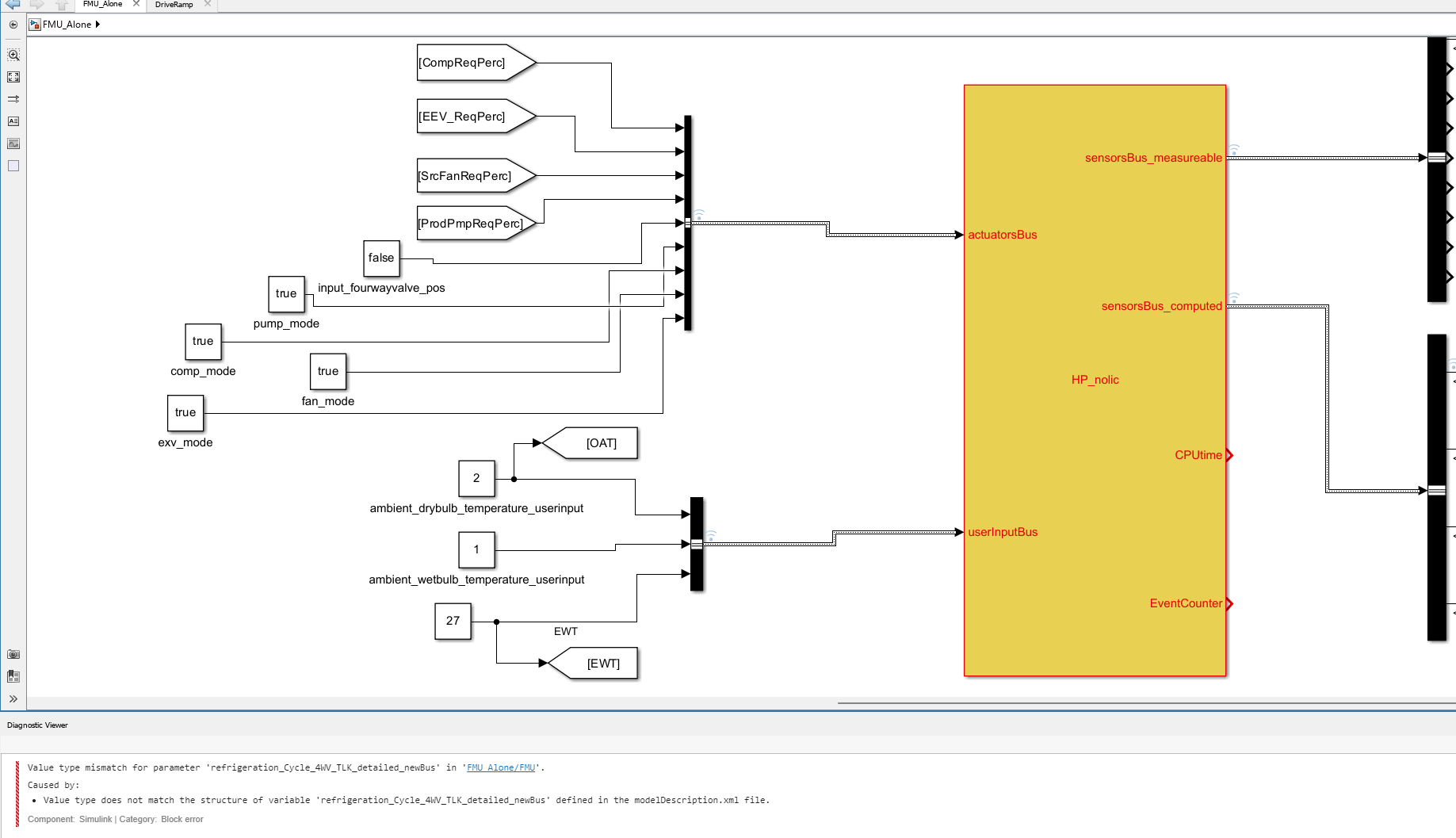
About Discussions
Discussions is a user-focused forum for the conversations that happen outside of any particular product or project.
Get to know your peers while sharing all the tricks you've learned, ideas you've had, or even your latest vacation photos. Discussions is where MATLAB users connect!
Get to know your peers while sharing all the tricks you've learned, ideas you've had, or even your latest vacation photos. Discussions is where MATLAB users connect!
More Community Areas

MATLAB Answers
Ask & Answer questions about MATLAB & Simulink!

File Exchange
Download or contribute user-submitted code!

Cody
Solve problem groups, learn MATLAB & earn badges!

Blogs
Get the inside view on MATLAB and Simulink!
AI Chat Playground
Use AI to generate initial draft MATLAB code, and answer questions!