Pull up a chair!
Discussions is your place to get to know your peers, tackle the bigger challenges together, and have fun along the way.
- Want to see the latest updates? Follow the Highlights!
- Looking for techniques improve your MATLAB or Simulink skills? Tips & Tricks has you covered!
- Sharing the perfect math joke, pun, or meme? Look no further than Fun!
- Think there's a channel we need? Tell us more in Ideas
Updated Discussions

In MATChess, you play chess against MATLAB with only your mouse click. MATLAB plays white and moves first. You play the dark pieces. Click a piece, then click a green square. That is all you need.
The goal is not just to move pieces. It is to think one step ahead of MATLAB, and to choose the level that matches your skill.
Play the game
Entry page: MATChess
Open the entry, click Play Game, then click Run this app in MATLAB Drive.
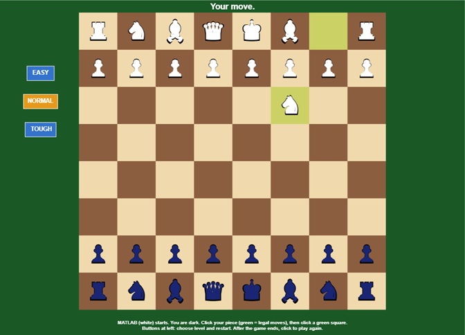
The start of a game. MATLAB (white) has made its first move. Now it is your turn.
How to play
- MATLAB moves first. Wait until the top line says Your move.
- Click one of your dark pieces.
- Green squares show every legal move for that piece.
- Click a green square to make your move.
- When the game ends, click anywhere to play again.
The game only lets you make legal moves. You cannot make a move that leaves your own king in check.
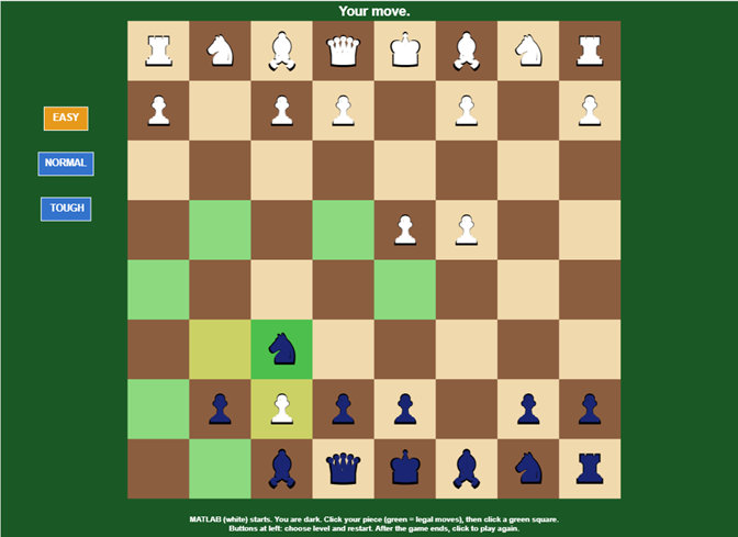
A dark knight is selected. Green squares show where it can go. Yellow squares show MATLAB's last move.
What the colours mean
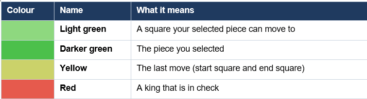
The line at the top tells you what is happening: Your move., CHECK! Your move., MATLAB is thinking..., or the result when the game ends.
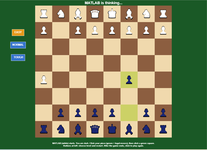
MATLAB is thinking. After your move, it waits half a second and then replies.
Choose your level
There are three buttons on the left side of the board: EASY, NORMAL and TOUGH. Click a button to start a new game at that level. The orange button shows the level you are playing. The game starts on NORMAL.
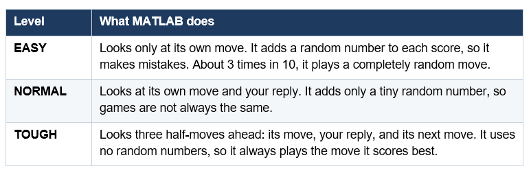
Try this: play the same first moves on EASY and on TOUGH. Where does MATLAB start to play differently?
How MATLAB chooses a move
MATLAB gives every position a score. A higher score is better for MATLAB. The score has three parts:
- Piece value: pawn 100, knight 320, bishop 330, rook 500, queen 900, king 20,000.
- Centre bonus: knights and bishops get extra points when they stand near the centre of the board.
- Pawn push: pawns get extra points as they move forward.
Then MATLAB tries its moves and your replies, and keeps the move with the best score. It looks at captures first, so it can skip weak moves faster. This idea is called alpha-beta pruning. The king is worth so much that losing it ends the search, and a quicker win scores a little higher.
The rules in the game
Included:
- All normal moves for every piece.
- Pawns can move two squares from their first row.
- Check, checkmate and stalemate.
- A pawn that reaches the last row becomes a queen.
Not included:
- Castling and en passant.
- Draw by repetition and the 50-move rule.
- Choosing a piece other than a queen when a pawn is promoted.
One click does every job
The game uses just one input: a click. Each click does one job, depending on where you click and what is happening:
- Click a level button: start a new game at that level.
- Click one of your pieces: select it.
- Click a green square: move the selected piece.
- Click after the game ends: play again.
Each square is 66 pixels wide. The game turns the click position into a column and a row with ceil((x-136)/66) and ceil((y-50)/66). After the game ends, it waits half a second before it accepts a click. This stops a quick click from hiding the result.
How the board is drawn
The board is stored as an 8-by-8 matrix. Positive numbers are MATLAB's white pieces and negative numbers are your dark pieces. The numbers are 1 pawn, 2 knight, 3 bishop, 4 rook, 5 queen, 6 king, and 0 for an empty square. A move is four numbers: the start row and column, and the end row and column.
The code is split into three parts: initialize, update and render. The graphics are created once and then reused. The board is one patch object with 64 squares, and only the colours change from frame to frame. The pieces are Unicode chess symbols in text objects. Each piece is drawn twice: a bigger black symbol behind and a smaller coloured symbol on top. This gives every piece a dark outline.
Try this
- Can you beat TOUGH? How many moves does it take?
- Play on EASY and try to catch MATLAB's random mistakes.
- Can you trap a piece with a knight fork?
Which level can you beat? Tell me in the comments. Thank you for playing!

Tips and Tricks from a One-Button Robot Game
Kinematix 3D is my STEM entry in the MATLAB One Button Game Mini Hack: a pick and deliver robot arcade game you play with a single button. Tap once to send the arm to the object, tap again to deliver it to the target, and finish three missions to set your score. Behind thst one button is real robotics: forward and inverse kinematics, smooth motion planning, a seven state game machine and a fast 3D animation loop, all in plain MATLAB with no toolboxes. This live script walks through the ten tricks that make it work. Each tip has runnable code, a 3D figure with a caption tying it back to the game, and links to the Mathworks documentation for every function used. Try the game first, then see how it works.
PLAY KINEMATIX 3D
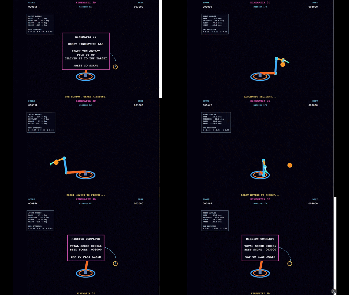
Tip 1-Organize Robot Parameters
Trick: Store the robot's link lengths in one vector instead of defining each link seperately.
L=[0.8 0.65 0.35];
Why it works: The vector makes the three link dimensions easy to access and reuse throughout the robot's forward and inverse kinematics calculations.
Practical Takeaway: Keep robot dimensions centralized so you can modify the robot geometry without rewriting the calculations.
Tip 2-Forward Kinematics with Cumulative Joint Angles
Trick: Calculate each link's orientation by accumulating the preceding joint angles.
a=q(2);
b=q(2)+q(3);
c=q(2)+q(3)+q(4);
Why it works: Each link's orientation depends on the combined rotation of the joints before it. Cumulative angles simplify the forward kinematics equations.
Practical takeaway: Calculate joint angle sums once and reuse them instead of repeating the expressions throughout your code.
Tip 3-Calculate the End-Effector Radius
Trick: Project each robot link onto the horizontal plane to calculate the arm's radial reach.
r=L(1)*cos(a)+L(2)*cos(b)+L(3)*cos(c);
Why it works: Each cosine calculates a link's horizontal contribution,and their sum gives the robot's total radial distance from its base axis.
Practical takeaway: Calculate the radial each once,then reuse it to determine the end effector's X and Y coordinates.
Tip 4-Convert Radical Reach into Cartesian Coordinates
Trick: Use the base joint angle to convert the robot's radial reach into its X and Y positions.
x=r*cos(q(1));
y=r*sin(q(1));
Why it works: The base rotation q1 resolves the radial distance into two perpendicular horizontal components.
Practical takeaway: Use polar to Cartesian conversion to position the robot accurately in 3D space.
Tip 5-Calculate Vertical End-Effector Position
Trick: Sum the vertical contribution of each robot link and the base height.
z=h+L(1)*sin(a)+L(2)*sin(b)+L(3)*sin(c);
Why it works:Each sine term calculates a link's vertical contribution.
Practical takeaway: Combine horizontal and vertical coordinates to determine the end-effector's 3D position.
Tip 6-Solve the Inverse Kinematics with the Law of Cosines
Trick: Calculate the elbow angle from the desired wrist position.
c3=(rw^2+zw^2_L(1)^2-L(2)^2)/(2*L(1)*L(2));
Why it works: The law of cosines determines the elbow configuration needed to reach the target.
Practical takeaway: Use geometric relationships to calculate joint angles instead of guessing positions.
Tip 7-Calculate the Base Rotation
Trick: Determine the base joint angle from the target's horizontal coordinates.
q1=atan2(p(2),p(1));
Why it works: atan2 determines the correct angular direction while accounting for the coordinate quadrant.
Practical takeaway: Use atan2 for reliable angular calculations in robotics.
Tip 8-Interpolate Smooth Joint Motion
Trick: Use smoothstep interpolation to avoid abrupt movement between joint positions.
s=3*u^2-2*u^3;
Why it works: The interpolation begins and ends with zero slope, producing smoother transitions.
Practical takeaway: Smooth joint trajectories improve the visual quality of robot animation.
Tip 9-Detect a New One Button Press
Trick: Detect the transition from an unpressed button to a pressed button.
tap=pressed(k) && ~pressed(k-1);
Why it works: Comparing consecutive input states detects a new press rather than repeatedly registering a held button.
Practical takeaway: Use edge detection for precise one button game controls.
Tip 10-Calculate the Wrist Joint Angle
Trick: Calculate the wrist angle needed to maintain the fixed tool angle.
q4=phi-q2-q3;
Why it works: The wrist compensates for the shoulder and elbow rotations to maintain the specified tool angle.
Practical takeaway: Coordinate joint angles to control the end effector's tool orientation.
MATLAB Functions Used in KINEMATIX 3D Robot
KINEMATIX 3D ROBOT uses MATLAB's built in mathematical and programming functions to calculate robot geometry, solve inverse kinematics, and animate joint movement. Functions such as cos, sin,atan2, hypot,and acos handle trignometric calculations and coordinate transformations, while robotFK calculates forward kinematics. Smoothstep interpolation controls motion between joint configurations, and logical operations manage one-button input and game state transitions. Together, these functions connect mathematical robotics principles with interactive 3D simulation.
Advanced 3D Robotics Visualization -From Mechanical Design to Mathematical Intelligence
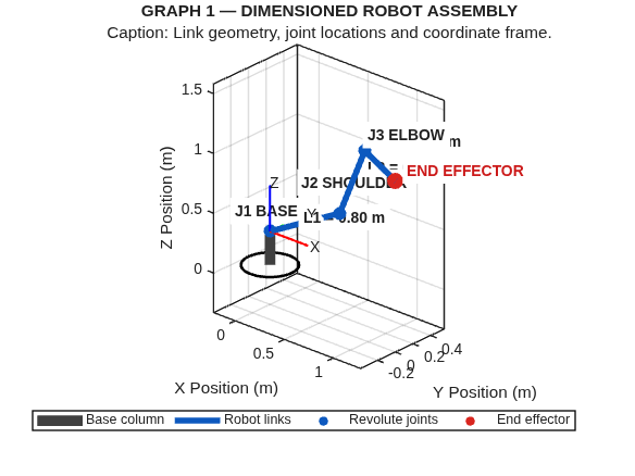
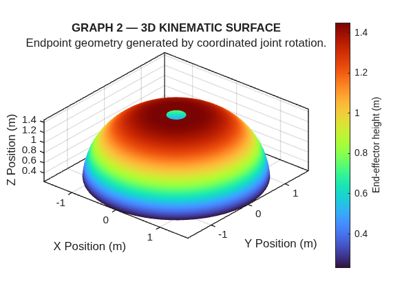
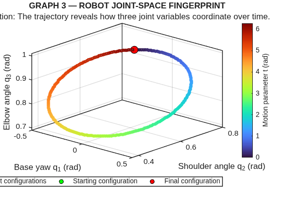
The final stage of KINEMATIX 3D brings the robot's engineering principles together through three complementary visualizations. The first presents the robotic arm as a dimensionec mechanical assembly, identifying its links, joints, coordinate frame, and end-effector. The second uses a 3D kinematic surface to reveal how joint rotations shape the robot's reachable positions. The third introduces a joint-space fingerprint, showing how multiple joint variables coordinate throughout a movement space.
Together, these visualizations connect mechanical engineering, spatial geometry, and computational mathematics. They demonstrate that robotics is not simply about making a machine move; it is about understanding the relationships that make controlled movement possible.
Why this belongs at the end: It transforms the earlier MATLAB tips and equations into visible engineering results, giving readers an opportunity to see how individual programming techniques and MATLAB STEM education contribute to a complete robotic system.
run('KINEMATIX_3D_Engineering_Gallery.mlx')

How to Play
In Circuit Runner, your goal is to make your way through a series of logic gates while staying ahead of the glitch chasing you.
Each gate has a set of binary inputs, either 0 or 1. Work out what the output should be and press when the scanner highlights the correct path.
- Upper path: Output 1
- Lower path: Output 0
Your first press locks in your answer for that gate, so make sure the correct path is highlighted before pressing.
If you choose the wrong path or fail to answer in time, your signal gets jammed, allowing the glitch to catch up. Keep getting the answers right to stay ahead!
STEM Concept: Boolean Logic
Boolean logic is the basis of how digital circuits work. It uses two possible values, 0 and 1, which can also represent false and true.
Logic gates take one or more binary inputs and produce an output based on a particular rule.
For example, an AND gate only produces an output of 1 when both its inputs are 1. An OR gate, on the other hand, produces 1 when at least one input is 1.
In this game, you'll come across different gates and need to quickly figure out their outputs. This is the same process used to construct truth tables in digital logic.
Timing Your Press!
You'll need to think quickly as the game progresses.
- Read the gate and its inputs as soon as they appear. Try to work out the output before looking at the scanner.
- The scanner starts at 0 for every new gate and switches between the two paths. Press when it highlights your answer.
- As you move through the stages, the scanner switches faster and the gates approach more quickly, giving you less time to decide.
- Try to get three correct answers in a row to activate a two-second speed boost. Every correct answer also helps you get further ahead of the glitch.
Getting an answer wrong temporarily jams your signal, so it's worth checking your answer rather than pressing too early.
Logic Gate Reference
Here's a quick reference for the gates you'll encounter:
- AND: Outputs 1 only when both inputs are 1.
- OR: Outputs 1 when at least one input is 1.
- NOT: Reverses the input. If the input is 0, the output is 1, and vice versa.
- XOR: Outputs 1 when the two inputs are different.
- NAND: Outputs 1 when at least one input is 0.
- NOR: Outputs 1 only when both inputs are 0.
- XNOR: Outputs 1 when both inputs are the same.
A useful way to remember the gates is that NAND, NOR and XNOR are simply the opposites of AND, OR and XOR respectively.
If you're unsure about a gate, try thinking about when its output would be 0 instead.
How It Works in MATLAB!
The game uses MATLAB's logical operations to calculate the correct output for each gate.
At the start of each stage, the available gate types are shuffled to give you a different sequence of questions.
The game continuously updates the scanner as it switches between the two paths. When you press, MATLAB locks in the output that was highlighted on the last displayed frame and checks it against the correct answer.
The graphics are updated throughout the game to show the track, scanner position, score and distance from the glitch.
As you play, try to get familiar with the different gates rather than calculating each output from scratch. Once you recognise their patterns, answering becomes much faster, which is exactly what you'll need in the later stages.
How to Play
The goal of Descent is to move the ball to the lowest point of the curve using gradient descent.
Watch the moving meter and press to select a learning rate. Each press moves the ball one step and uses up one move.
To complete a stage, you need to get within 0.06 of the target position before running out of moves. If the ball moves outside the plotted range, the game ends.
STEM Concept: Gradient Descent
Gradient descent is a method used to minimize a function, such as the loss function used when training machine learning models.
In this game, the slope of the curve tells you which direction to move, while the learning rate controls how far you move in that direction.
- A small learning rate gives you smaller steps, which are safer but may take longer to reach the minimum.
- A large learning rate gives you bigger steps, which can get you there faster but may also cause you to overshoot.
The challenge is to choose a learning rate that gets you close to the minimum without taking unnecessary steps.
Choosing a Learning Rate
Use the tangent line to understand the slope at your current position. After each move, check the loss value to see whether your choice helped.
For the first three stages, the meter is colour-coded:
- Cyan: Moves you closer to the minimum quickly.
- Amber: May overshoot the minimum but can still reduce the loss.
- Red: May increase the loss instead of reducing it.
The last two stages have a neutral meter, so you'll need to judge the learning rate using the curve and the feedback from your previous moves.
A Few Hints for Each Stage :)
- First Contact: Try a learning rate of 1.000.
- The Steep Valley: The curve is steeper, so try a smaller rate of 0.250.
- Low Gravity: The slope is gentler, so a larger rate of around 3.333 works well.
- Shifted Reality: Try aiming for 0.625.
- The Final Descent: Start with smaller steps where the curve is steep. As you get closer to the minimum, you can try increasing the learning rate.
In the first four stages, the loss function has the form:
Loss = a * (x - target)^2 + minimumLoss
For these curves, a learning rate of 1 / (2 * a) will take you directly to the minimum in one step.
Try to finish each stage with as many moves remaining as possible to earn a higher score!
How It Works in MATLAB
Every time you press, the game updates the ball's position using the gradient descent rule:
x_new = x - alpha * gradient
Here, x is your current position, alpha is the learning rate you selected, and gradient is the slope of the curve at that position.
MATLAB calculates the gradient from the derivative of the loss function and moves the ball to its new position.
The final stage uses a slightly more complicated function with a quartic term. This means the learning rate needed to reach the minimum in one step changes depending on your current position.
As you play, try experimenting with different learning rates and observe how they affect the ball's movement and the loss. The idea is to get a feel for why choosing the right learning rate matters when using gradient descent.

My fourth entry, Big Wave (entry 16646), drops you on a breaking wave at sunset. Your surfer carves up and down the face on their own. You tap at the bottom of each turn to pump for speed, stay ahead of the curl chasing you, and launch airs off the lip when your board turns gold.
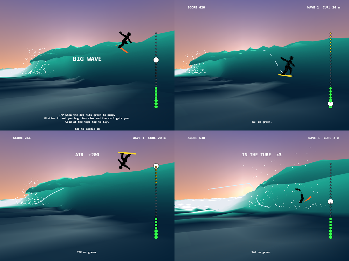
Real frames from the game: the title screen, a pump, an air, and riding inside the barrel for triple points.
As with my other entries, I built it with help from an AI coding assistant (Claude Code) and tested every change in MATLAB. This one took four playtests to get right, and most of what I learned came from the ones that didn't work.
1. One button is a timing game, not a tapping game
The wave looked good from the first version. The gameplay didn't.
- Version 1: tapping switched the surfer between climbing and dropping. My playtest verdict: it played like Flappy Bird, where you keep pressing until something happens.
- Version 2: two lines, high and low, with rocks and breaking lips to dodge and a camera that swung around to look ahead. It was worse. The hazards were hard to read, the new camera lost the barrel view, and it still wasn't fun.
- Version 3: the surfer carves by themselves, and you only tap to pump at the bottom of a turn. The closer to the exact bottom, the more speed you get. A tap at any other moment bogs the board down and costs a quarter of your speed, so mashing is punished.
Two later changes made version 3 work. First, every turn now has a random length, so you watch the turn instead of tapping to a beat. Second, the cue moved from a ring on the surfer, which got lost in the scene, to a fixed gauge on the right: a white dot rides a column of dots, green at the bottom for a pump and gold at the top when you can fly.
To check that skill matters, I ran bots through the final version. Idling and spamming die within seconds, and only good timing keeps you alive:

Median of 8 runs per bot. Going for airs scores about 2.5 times more than playing safe, but it dies sooner. That trade-off is the choice I wanted.
Bots can't tell you whether something is fun, but they do catch the worst designs before a playtest.2. A breaking wave from three keyframes and one matrix product
The wave is a single surf. Each slice across it is a cross-section with 13 control points, blended from three keyframes: an open face, a curling barrel, and collapsed whitewater. The blend depends on how far that slice is from the curl, so the wave throws a barrel just ahead of the curl and turns to foam behind it.
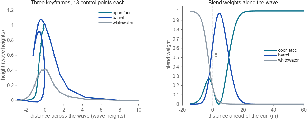
The useful trick is that a cubic spline is linear in its data. Interpolating the identity matrix once gives a matrix that splines any set of control points:
t = [1:.5:3.5 linspace(4,12,30) 12.5 13]; % where to sample the curve
S = spline(1:13,eye(13),t)'; % 40 x 13 spline matrix, built once
Each frame, the control points for all 64 slices are a weighted mix of the keyframes, and S*CX smooths every slice in one matrix product. There are no loops and no spline calls per frame.3. A 24 x 28 sprite in 112 characters
The surfer started as a stick figure. I wanted a proper silhouette, but imread is banned and the entry has to be a single file, so I drew the sprite from thick limb segments in a helper script and packed it into the code as text. Each character stores 6 pixels:
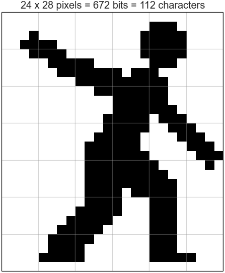
c = dec2bin(double('0000003P407`?07`7P7`...')-48,6)'; % 112 chars -> 672 bits
[j,i] = find(reshape(c-48,24,28)); % filled pixels
px = [j-12 28.5-i]'*.07; % pixel offsets in metres
The pixels are drawn as one scatter3 of square markers. They're placed in the camera's screen plane, so the sprite always faces you, and a 2-by-2 rotation leans it into each carve and flips it during an air:
o = .2*sin(s.ph)+2*pi*a/.9*(s.air > 0);
body = P+[r' u']*[cos(o) -sin(o);sin(o) cos(o)]*px; % r, u: screen right and up
As a bonus, the scatter sprite rendered faster than the old stick figure. Frame time dropped from about 40 ms to 15 ms on my PC.4. A HUD that stays put in a 3D scene
Waves grow as you progress, so the camera position and target are both multiplied by the wave height H. Anything else placed at H times a fixed point therefore stays at the same spot on screen. The gauge uses this: its dots sit a little in front of the camera, offset along the screen's right and up vectors, and never move however big the wave gets:
c = [3 1.6 .3]; f = [.3 -1.2 .45]-c; f = f/norm(f); % camera position and view direction
r = cross(f,[0 0 1]); u = cross(r,f); % screen right and up
P = H*(c+f+.5*r-.3*u+g*.17*u); % g: each dot's place on the gauge
The same right and up vectors stand the sprite upright.5. Squeezing in the last characters
The final file counts exactly 10,000 of 10,000 characters. The counter reformats your code first, so comments are free but every space around a comma or operator counts, as I described in my first post. Long lists of numbers are expensive for that reason, so:
- Pack number tables as strings. The keyframe control points are multiples of 0.05, so each one fits in a single character:x = reshape(double('\\`YMZVCUTHPQRKNZFIW>00(')/20-4.6,3,8);
- Swap an FFT ocean for a dozen sine waves. My first version had a full Tessendorf FFT ocean for the small chop. Twelve sine wave trains, each moving at its own deep-water speed sqrt(9.81*k), look nearly the same at this scale and cost far fewer characters.
- Use deal to reset state. [s.ys,s.pts,s.air,s.dead] = deal(0); resets many fields in one statement.
- Find a short path for the colour. One scalar colour index through a custom colormap (haze, deep blue, backlit aqua, foam) was shorter and about twice as fast as a full RGB CData.
Play it
If MATLAB Online is slow for you, run it in desktop MATLAB: download the starter project, copy the entry's code into game.m, and run minihackContest.play.
How long can you outrun the curl?

There are almost 200 creative and fun One-Button Games created in this year’s Mini Hack contest. Play them, vote for your favorites, and win MathWorks prizes!
We’re giving away 20 MathWorks T-shirts or pairs of socks to community members who play and vote. And here’s the fun part: The more games you play and vote for, the higher your chance of winning!
Not sure where to start? Here are a few games to get you going.
Just for fun
Play & Learn
❤ Your Votes Matter
Behind every game is a community member who spent time imagining it, building it, testing it, and sharing it with all of us.
A vote is a simple way to say: “I played your game. I enjoyed it. Nice work!”
So play a few. Vote for your favorites. Then maybe play a few more.

I wanted to read a grid child’s Position immediately after resizing its parent. Sometimes drawnow returned while the child still had its old size. A second read, with no further changes to the figure, gave a different rectangle.
A MATLAB uifigure has a browser-based client that computes grid layout and reports the resulting positions back to MATLAB. So when can MATLAB code read the updated values? In the layouts I tested, a wait inside that client gave me the same Position values as a later read. The wait starts with 220 ms without a container resize notification, then lets the client finish the layout work it has queued.
This post is an abridged English adaptation of my own article on Qiita (in Japanese). I used AI assistance to prepare the English write-up and reproduction files.
Caution: This trick relies on undocumented, private MATLAB internals. It was verified only by testing on Windows and may stop working in any release.
Why a position can change after drawnow
The uigridlayout documentation mentions that a child’s Position may lag when it is added to a grid. I saw the same kind of lag when resizing an existing grid. MATLAB updates the component properties as position change events arrive from the uifigure client. A read can occur while the client still has another relayout pending.
In the Windows releases I inspected (R2023a through R2026b), the Grid Layout controller used a 200 ms Lodash throttle for parent resize events, with both leading and trailing calls enabled. The first resize can run immediately. If another comes in during that interval, the trailing call can run on a timer, using the latest resize. If the grid contains another resizable container, that relayout can trigger another resize further down the tree.
The internal ViewModel method stabilize() waits for registered asynchronous work. The trailing timer hasn’t registered a relayout yet, so the ViewModel can report that its current work is done while the timer is still pending. A single requestAnimationFrame can also run before that timer fires.
How I waited for updated positions
Update: I’ve released waitForFigureLayout as a standalone utility to make it easier to use in your own apps. You can download the packaged version from MATLAB Central File Exchange.
Run JavaScript in the uifigure client
Reaching that window through the figure's hidden Controller follows the approach Yair Altman described in Customizing uifigures on Undocumented MATLAB. In the releases I tested, the window is on the controller's PlatformHost rather than its Container. The code registers a listener on the figure's ViewModel, then calls executeJS on that window. The JavaScript sends a completion event through the ViewModel after waiting for the layout. These steps use private APIs and require a figure whose host exposes a CEF window.
On Windows, use an ordinary uifigure from R2023a through R2024b. To use the same code in the desktop from R2025a through R2026b, create a separate figure window with the undocumented matlab.ui.internal.uifigureIsolated. Use fig = matlab.ui.internal.uifigureIsolated; in place of fig = uifigure; when creating the figure.
Wait for the grid’s resize work
- Wrap emitContainerResizeControllerEvent on the figure’s container controllers. Record the time of the most recent resize notification and keep that timestamp across waits. When installing a new hook, start the quiet period afresh because earlier notifications may have been missed.
- Wait for 220 ms without another notification. That is the Grid Layout controller’s 200 ms throttle interval plus a 20 ms margin. Each resize restarts the quiet period, so nested relayouts have time to schedule their own work. Give up after three seconds of continued activity.
- Await stabilize() when it exists, then wait one animation frame. In R2023a and R2023b, the grid relayout itself was scheduled as an animation-frame callback. In R2024a and later, the relayout was registered with the ViewModel.
- Send the completion event through the figure’s ViewModel so that it follows position notifications already dispatched on that channel. On receipt, read the MATLAB properties.
The 220 ms interval is derived from the throttle in the implementation I inspected. Both the throttle interval and the private APIs can change between releases.
Validation
I used a panel containing a two-row grid with a 'fit' label above a tab group. The second tab contained a nested grid and label. After the initial layout had settled, I measured a second wait and compared the outer label’s and tab group’s Position and the nested label’s getpixelposition(...,true). I took the first reading after the wait and a drawnow, and the second 0.5 seconds later.
In interactive MATLAB desktop sessions on Windows, I ran six trials per scenario in each release from R2023a through R2026b. All three rectangles agreed in all 192 trials.
The per-release median waits ranged from 241 to 249 ms after resizing the panel, enlarging the fit-row label, switching tabs, and enlarging the nested label. They ranged from 233 to 246 ms after only the panel resize and label enlargement, and from 296 to 375 ms after two panel resizes 50 ms apart. With no change, the wait took 8 to 12 ms.
The attached layoutWaitDemo.zip contains a smaller reproduction fixture, a single grid whose parent is resized twice within the throttle interval, and the same waitForFigureLayout.m and waitForFigureLayout.js shown below. To compare drawnow alone with the browser wait, extract the ZIP and run this command from the extracted folder.
matlab -batch "layoutWaitDemo(false, 8); layoutWaitDemo(true, 8)"
In this smaller fixture on Windows R2023a, R2024b, and R2026b, each release showed a position change after the first read in 8/8 baseline runs and 0/8 runs with the browser wait. The median extra waits were 362, 375, and 377 ms, respectively.
Using the wait in your own code
Save the two blocks below as waitForFigureLayout.m and waitForFigureLayout.js in the same folder and put that folder on the MATLAB path. Call the function once before editing the layout to install the resize hooks. After making your changes, call it again before reading Position. Keep the figure visible while waiting for the animation frame.
fig = uifigure;
panel = uipanel(fig, "AutoResizeChildren", "off", "Position", [20 20 300 250]);
grid = uigridlayout(panel, [1 1]);
child = uilabel(grid, "Text", "Grid child");
drawnow
waitForFigureLayout(fig); % Install hooks before the first layout change.
panel.Position(3:4) = [400 300];
drawnow
waitForFigureLayout(fig); % Wait for the queued resize work and its reply.
drawnow
position = child.Position
MATLAB file: waitForFigureLayout.m
function waitForFigureLayout(fig)
% waitForFigureLayout Dispatch the browser wait and receive its result on the figure ViewModel.
arguments (Input)
fig (1, 1) matlab.ui.Figure
end
% Find the browser window that hosts the figure.
% struct() reads every hidden property, so besides MATLAB:structOnObject it can
% emit unrelated deprecation warnings (JavaFrame, GraphicsSmoothing, ...).
% Silence all warnings only for these three calls.
warningState = warning("off", "all");
warningCleanup = onCleanup(@() warning(warningState));
figureData = struct(fig);
controller = struct(figureData.Controller);
host = struct(controller.PlatformHost);
clear warningCleanup
assert(isfield(host, "CEF") && ~isempty(host.CEF), ...
"This figure has no CEF window. Use uifigure through R2024b. " + ...
"In R2025a or later, create the figure with matlab.ui.internal.uifigureIsolated.");
viewModel = controller.ViewModel;
% Use a unique completion event for this request and subscribe before dispatch.
requestId = erase(string(java.util.UUID.randomUUID()), "-");
eventName = "FigureLayoutWaitCompleted_" + requestId;
reply = [];
listener = viewModel.addEventListener(char(eventName), @receive);
listenerCleanup = onCleanup(@() delete(listener));
configuration = struct("figureId", string(viewModel.getId()), ...
"channel", string(matlab.ui.internal.FigureServices.getUniqueChannelId(fig)), ...
"eventName", eventName);
source = fileread(fullfile(fileparts(mfilename("fullpath")), "waitForFigureLayout.js"));
script = replace(string(source), "__LAYOUT_WAIT_CONFIGURATION__", string(jsonencode(configuration)));
host.CEF.executeJS(char(script), 10);
% Yield to MATLAB callbacks and bound the wait for a missing browser reply.
clock = tic;
while isempty(reply) && toc(clock) < 8
pause(0.01);
end
assert(~isempty(reply), "Timed out waiting for the figure ViewModel reply.");
if isfield(reply, "error")
error("Browser layout wait failed: %s", string(reply.error));
end
clear listenerCleanup
function receive(~, event)
% receive Store the payload for this request's completion event.
reply = event.data;
end
end
JavaScript file: waitForFigureLayout.js
(config => {
const delay = milliseconds => new Promise(resolve => setTimeout(resolve, milliseconds));
require(["viewmodel/impl/ViewModelManagerFactory", "MW/componentframework/ControllerService"],
async (factory, service) => {
const managers = Object.values(factory._viewModelManagerCache)
.filter(manager => manager.hasById(config.figureId));
if (managers.length !== 1) {
throw new Error("Expected one ViewModel manager for this figure.");
}
const manager = managers[0];
const viewModel = manager.getById(config.figureId);
const send = result => viewModel.dispatchEvent(config.eventName, viewModel,
result);
try {
// Keep resize timestamps across calls in this demo figure.
const resize = viewModel.figureLayoutWaitResize ??= {
last: performance.now(), hooked: new WeakSet()
};
const cache = service.getInstance(config.channel)._controllerCache;
const controllers = cache instanceof Map ? [...cache.values()] : Object.values(cache);
let watched = 0;
for (const controller of controllers) {
const original = controller?.emitContainerResizeControllerEvent;
if (typeof original !== "function") continue;
watched++;
if (resize.hooked.has(controller)) continue;
controller.emitContainerResizeControllerEvent = function (...args) {
resize.last = performance.now();
return original.apply(this, args);
};
resize.hooked.add(controller);
resize.last = performance.now();
}
if (watched === 0) throw new Error("No resize emitters found.");
// Let pending browser work run, then wait out the trailing resize timer.
document.body.getBoundingClientRect();
await delay(0);
const started = performance.now();
while (performance.now() - resize.last < 220) {
if (performance.now() - started >= 3000) {
throw new Error("Resize activity did not settle within 3 seconds.");
}
await delay(10);
}
// Drain registered layout work where supported, then wait one frame.
const root = manager.getRoot();
if (typeof root.stabilize === "function") await root.stabilize();
await new Promise(resolve => requestAnimationFrame(resolve));
send({ completed: true });
} catch (error) {
send({ error: String(error) });
}
});
return config.eventName;
})(__LAYOUT_WAIT_CONFIGURATION__)
I'd rather not believe this far too hacky way is the only thing to do. Has anyone found a supported way to wait until a grid layout's updated positions are available on the MATLAB side? I'd also be interested in results from other platforms or nested layouts.

The MATLAB One-Button Game Mini Hack runs from November 2nd through November 29th, 2026! The challenge is to make a game that can be played with one button. I thought this would be a good opportunity to share some of the graphics and programming ideas behind Arcade, a collection of 15 games I developed in MATLAB using Claude Code and the MATLAB MCP Server.
Before the 2024 MATLAB Shorts Mini Hack, Tim Marston published his walkthrough of Little Nemo's airship. I learned a lot from Tim's article, and it inspired me to enter the contest. I hope that sharing some of what goes into these games might encourage a few more people to give it a try this time around as well.
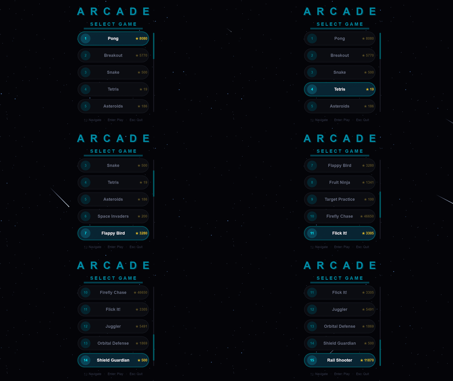
You can download Arcade from File Exchange or GitHub, add the project folder to the MATLAB search path, and run:
Arcade();
Creating and updating graphics
Arcade sports neon-styled graphics. This is accomplished by layering ordinary MATLAB graphics against a dark background. The bright colors used come from the shared GameBase palette, which enables the different games to keep a consistent appearance and accounts for quite a bit of that look.
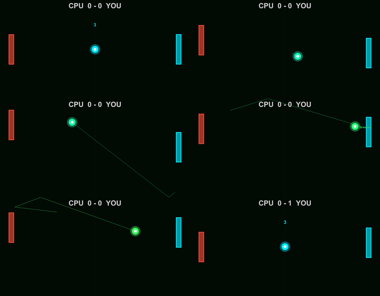
In Pong, the ball is made by drawing a colored dot, a semitransparent scatter marker and a smaller white dot at the same position. The ball and trail change from cyan through green, gold and red as the ball speeds up, while the center stays white. Against the dark background, these simple shapes give us the bright center and surrounding glow.
arcadeBallDemo();
worldSize = [854, 480];
position = worldSize / 2;
cyan = [0, 0.92, 1];
radiusParameter = max(3, round(min(worldSize) * 0.035));
baseCoreSize = 2 * radiusParameter;
baseDotSize = 5 * radiusParameter;
baseGlowArea = pi * (1.25 * radiusParameter)^2;
coloredDot = line(ax, NaN, NaN, ...
Marker=".", MarkerSize=baseDotSize, LineStyle="none", Color=[cyan, 0.15]);
glow = scatter(ax, position(1), position(2), baseGlowArea, cyan, "filled", ...
MarkerFaceAlpha=0.4);
core = line(ax, position(1), position(2), ...
Marker=".", MarkerSize=baseCoreSize, LineStyle="none", Color=[1, 1, 1, 1]);
ballLayers = {coloredDot, glow, core};
Here's how the ball looks as each layer is added:
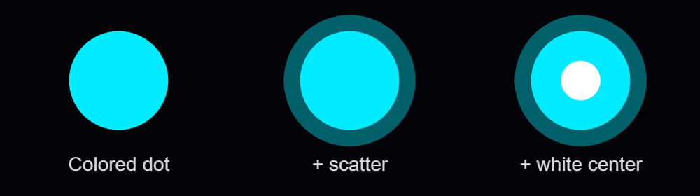
Setting NextPlot="add" preserves the existing graphics as we add the layers. Specifying the axes limits by using XLim and YLim keeps the view in place as the ball moves.
Each drawing call returns a handle to its object. With those handles stored in ballLayers, moving the ball involves assigning its new position to the existing objects:
for layerIndex = 1:numel(ballLayers)
ballLayers{layerIndex}.XData = position(1);
ballLayers{layerIndex}.YData = position(2);
end
drawnow
MathWorks' graphics-performance guidance recommends retaining graphics and updating the properties that change. Pong also checks whether its scores have changed before assigning new score text. Its trail uses preallocated position buffers, wrapping around as new positions arrive, and two retained lines display that history as a broad dim stroke with a narrower bright stroke.
Handling inputs using callback functions
The ball example responds to mouse presses through a callback function. After creating the scene, it assigns a function handle to the figure's WindowButtonDownFcn callback property:
fig.WindowButtonDownFcn = @reverseVerticalDirection;
MATLAB executes the callback function when a mouse button is pressed in the window. In the example, it is nested inside the local animateBall function:
function reverseVerticalDirection(~, ~)
velocity(2) = -velocity(2);
end
The two arguments supplied by MATLAB are the source object and event data. The ~ placeholders indicate that this function doesn't use them. As a nested function, it can access velocity in the enclosing function. Each mouse press reverses the shared vertical velocity, which the next loop iteration uses to move the ball.
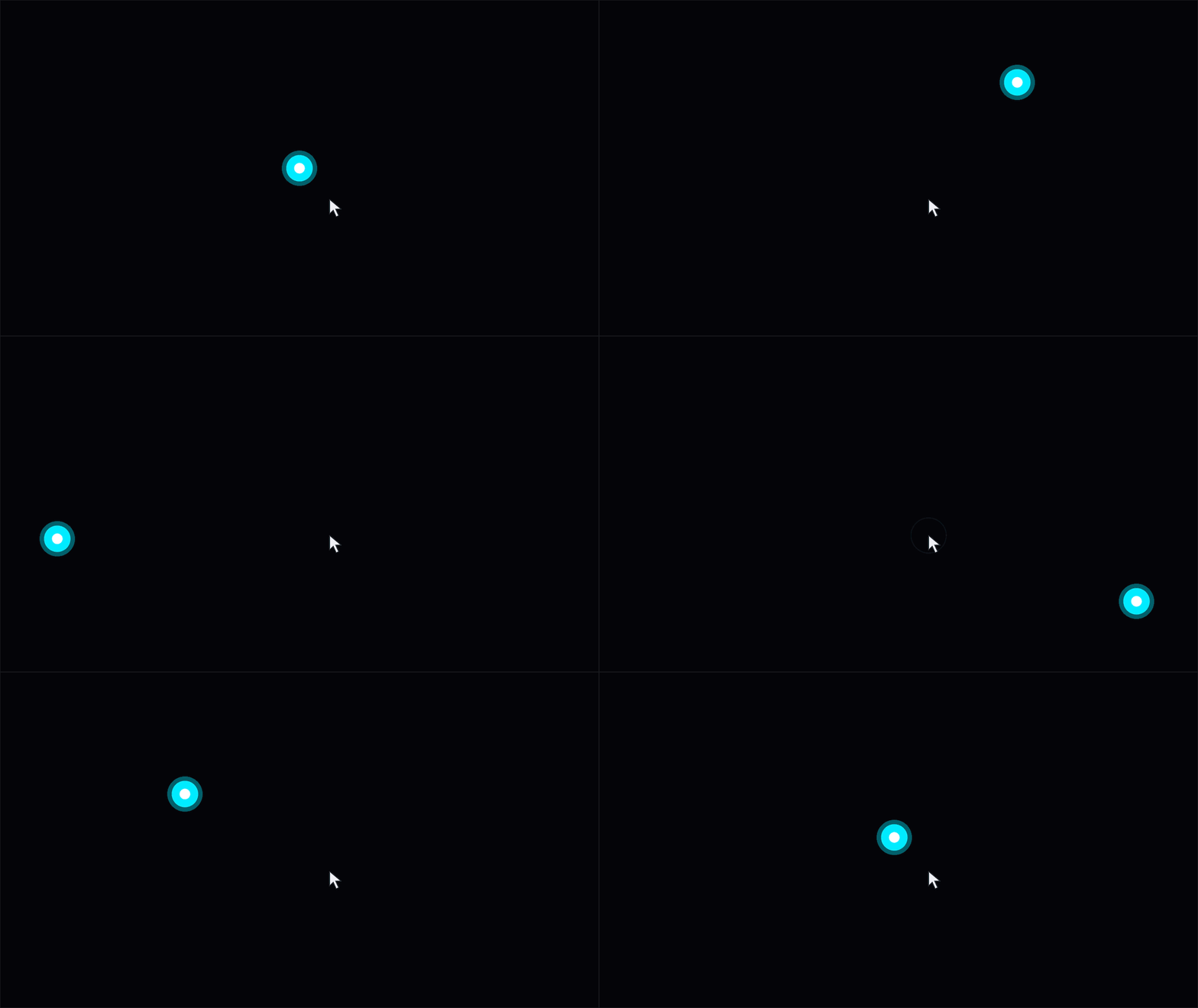
Arcade routes input through methods on the launcher. Its figure's KeyPressFcn callback property is assigned as follows, where obj is the launcher instance:
obj.Fig.KeyPressFcn = @(~, event) obj.onKeyPress(event);
The anonymous function forwards the event data to onKeyPress, where its Key property identifies the key. The launcher handles its own controls and passes appropriate input to the active game. Button release and scrolling have their own callback functions.
Mouse movement can control a paddle or aim a shot. To track the pointer as it moves within the figure, Arcade assigns a callback function to WindowButtonMotionFcn:
obj.Fig.WindowButtonMotionFcn = @(~, ~) obj.onMouseMove();
function onMouseMove(obj)
pointer = obj.Ax.CurrentPoint;
obj.MousePos = pointer(1, 1:2);
end
The axes' CurrentPoint gives the pointer position in game coordinates. MATLAB accounts for the axes' position and size, so the same code works when the playfield is resized or surrounded by margins.
On each game update, the launcher passes the stored position to the active game's onUpdate method. In Pong, obj now refers to the game instance. Once the incoming pos is available, its vertical coordinate determines the player's paddle position:
yLimits = obj.DisplayRange.Y;
if ~any(isnan(pos))
obj.PlayerPaddleY = max(yLimits(1) + obj.PaddleHalfH, ...
min(yLimits(2) - obj.PaddleHalfH, pos(2)));
end
The min and max calls keep the paddle's center at least half a paddle height from either edge. Moving the pointer into a margin therefore leaves the whole paddle inside the playfield. The graphics update then applies that position to the existing paddle patches.
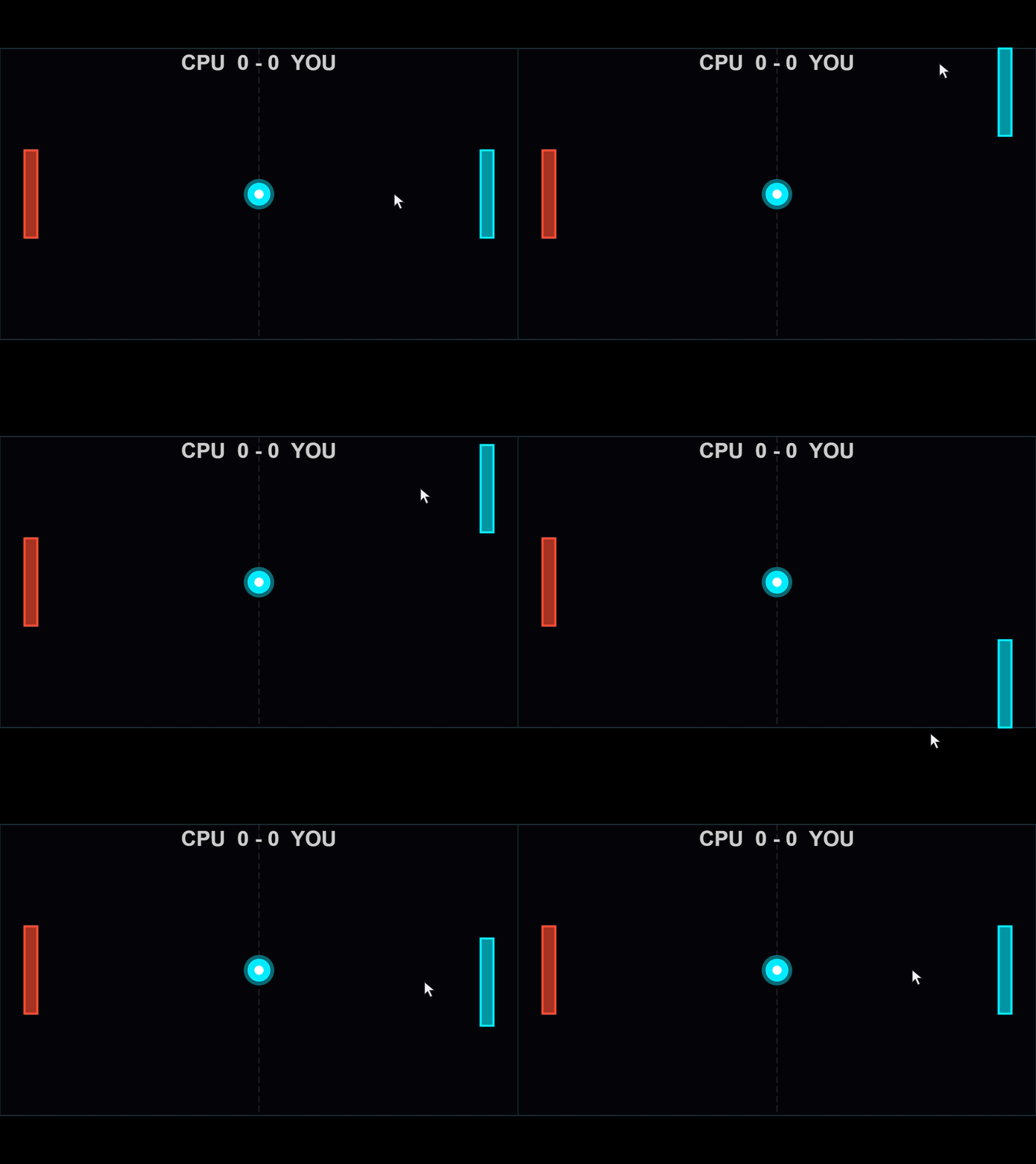
The animation loop's drawnow displays pending graphics changes and processes pending callbacks. Keeping callback functions short allows control to return to the loop promptly.
Animating visual effects
When the orb is launched in Flick It!, a call to spawnHitEffect creates a ring and rays that expand and fade. The launcher advances these shared effects alongside the active game.
In arcadeEffectsDemo.m, each click creates a burst at the mouse position, allowing several bursts to expand and fade together. To try it out, download the function, add its folder to the MATLAB path, and run:
arcadeEffectsDemo();
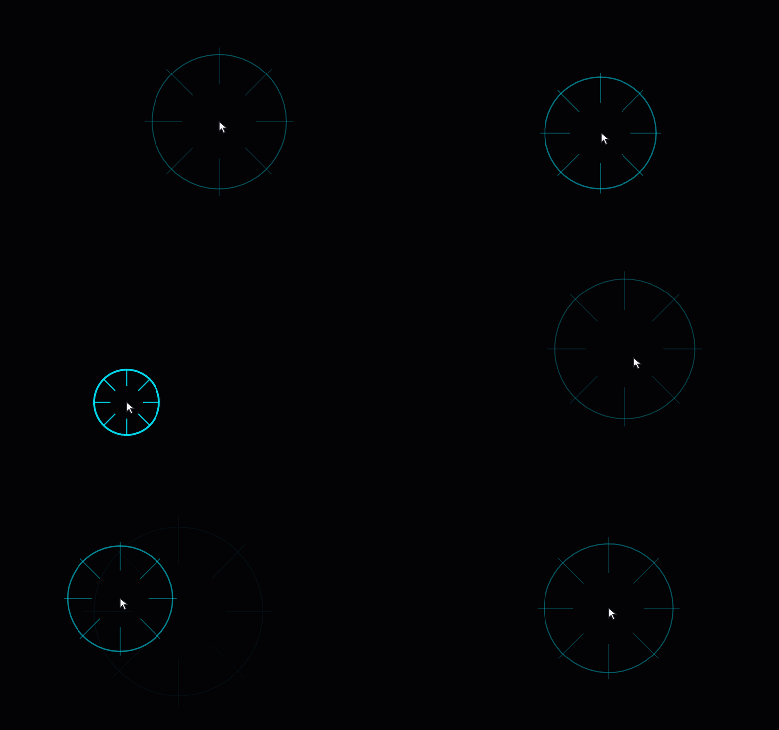
The nested callback function combines mouse-press handling with the mouse-position tracking introduced earlier. Here's the part that creates and stores a new burst:
fig.WindowButtonDownFcn = @createManualImpact;
function createManualImpact(~, ~)
point = ax.CurrentPoint;
position = point(1, 1:2);
if any(~isfinite(position)) || any(position < 0 | position > worldSize)
return
end
[newRing, newRays] = createEffect(position);
activeEffects(end+1) = struct('Ring', newRing, 'Rays', newRays, ...
'Center', position, 'AgeSeconds', 0, 'LastTime', toc(animationClock));
end
The bounds check ignores clicks outside the playfield. createEffect creates the lines, and activeEffects stores their handles, center and timing state. The animation loop updates each burst independently, allowing further clicks while earlier bursts are still expanding.
We can drive the geometry, transparency and line width from a common progress value: 0 when the burst begins and 1 at the end of its lifetime. Inside the function, the ring is updated as follows:
progress = ageSeconds / lifetimeSeconds;
eased = 1 - (1-progress)^2;
opacity = max(0, 1-1.5*eased);
ringRadius = radiusParameter * (1+2.5*eased);
ring.XData = center(1) + ringRadius*ringCos;
ring.YData = center(2) + ringRadius*ringSin;
ring.Color = [cyan, 0.8 * opacity];
ring.LineWidth = max(0.5, 3*(1-eased));
The ease-out expression starts the expansion quickly and slows it down toward the end. The burst fades out before its nominal lifetime finishes. ringCos and ringSin hold the circle's fixed directions, calculated before the loop. Arcade controls the transparency of these lines by assigning an RGBA value to Color, with alpha as the fourth component, ranging from 0 (clear) to 1 (fully opaque).
The row vectors rayCos and raySin contain the eight ray directions. Each ray joins the inner and outer radii, which increase as the burst expands:
innerRadius = radiusParameter * (0.5+1.5*eased);
outerRadius = radiusParameter * (1+3*eased);
for rayIndex = 1:numel(rays)
rays(rayIndex).XData = center(1) + [innerRadius, outerRadius]*rayCos(rayIndex);
rays(rayIndex).YData = center(2) + [innerRadius, outerRadius]*raySin(rayIndex);
rays(rayIndex).Color = [cyan, 0.6 * opacity];
rays(rayIndex).LineWidth = max(0.5, 2*(1-eased));
end
The lines are created when the burst begins, updated throughout its lifetime and deleted when it expires.
Display scaling: Keeping the scene in proportion
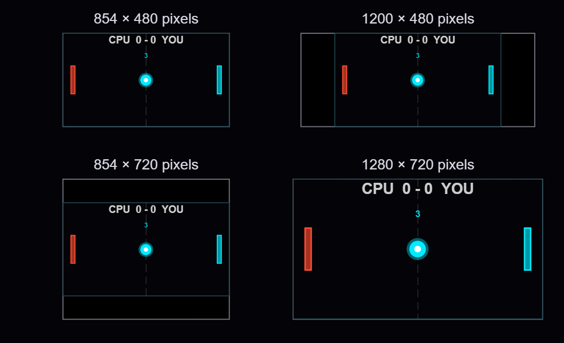
Try making the ball example's window wider while keeping its height the same. Space appears beside the playfield, and the ball still travels between the same boundaries. The example's reference window is 854 by 480 pixels, matching worldSize numerically. Resizing scales the playfield on the screen while the game's coordinate system remains unchanged.
The figure and axes use Units="pixels". Taking the min of the width and height ratios relative to the reference window gives the largest scale factor that fits in both directions. Applying that same scale to both dimensions preserves the playfield's 16:9 aspect ratio.
For a 1200-by-480 window, the height limits the scale to 1. The fitted area remains 854 by 480, leaving (1200-854)/2 = 173 pixels on each side. In a 1280-by-720 window, the playfield grows to approximately 1.5 times its reference width and height. Here are four window sizes at a common page scale:
MATLAB already scales graphics defined in data coordinates as the axes resize. For example, a paddle drawn with patch grows with the axes. In the example, marker sizes, font sizes and line widths use points, while scatter sizes use points squared.

To make a circle twice as wide, we need four times its area. Doubling SizeData multiplies its width by only √2:
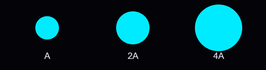
fig.SizeChangedFcn = @fitScene;
The nested fitScene callback function combines the axes calculation with these size updates:
function fitScene(~, ~)
if ~isgraphics(ax)
return
end
availableSize = max(fig.Position(3:4), [1, 1]);
displayScale = min(availableSize ./ worldSize);
fittedSize = worldSize * displayScale;
ax.Position = [(availableSize - fittedSize)/2 + 1, fittedSize];
% Always derive sizes from their reference values
core.MarkerSize = baseCoreSize * displayScale;
coloredDot.MarkerSize = baseDotSize * displayScale;
glow.SizeData = baseGlowArea * displayScale^2;
instruction.FontSize = baseFontSize * displayScale;
playfield.LineWidth = 0.5 * displayScale;
end
The first two entries of ax.Position set the left and bottom position, splitting the unused space equally between opposite sides. The last two give the fitted width and height. The axes limits remain unchanged, so movement and collision calculations keep using the same game coordinates.
At scale 1.5, the marker sizes are multiplied by 1.5 and the scatter area by 2.25. The updated sizes are calculated from their stored reference values. A 34-point reference marker becomes 51 points at scale 1.5, then 68 points at scale 2.
You can also use Units="normalized" to size and position the axes relative to the figure. Arcade's axes setup uses [0 0 1 1] to allocate the full available area:
obj.Ax = axes(obj.Fig, "Units", "normalized", "Position", [0 0 1 1]);
obj.Ax.XLim = obj.DisplayRange.X;
obj.Ax.YLim = obj.DisplayRange.Y;
Arcade's resize method obtains the available dimensions in pixels with getpixelposition and calculates the same display scale. It uses pbaspect to preserve the playfield's aspect ratio. MATLAB fits the playfield within the available space, leaving margins where needed:
axPx = getpixelposition(obj.Ax);
newPs = min(axPx(3) / 854, axPx(4) / 480);
gameAR = diff(obj.DisplayRange.X) / diff(obj.DisplayRange.Y);
pbaspect(obj.Ax, [gameAR 1 1]);
For Arcade, I also wanted markers, text and line widths to grow proportionally with the playfield. MATLAB also supports automatic resizing for text through FontUnits="normalized", which expresses font size as a fraction of the axes plot box height. This works well for text in a playfield with a fixed aspect ratio. Arcade's shared resize helper modifies current property values, using the ratio of the new scale to the previous scale; for example, moving from 51 to 68 points requires multiplying by 2/1.5. The function applies a common display scale to text, markers and line widths, in order to preserve their relative sizes as the window is resized.
FPS scaling: Let elapsed time determine the motion
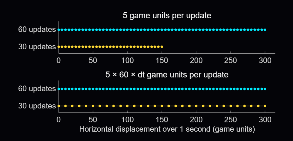
Suppose that the ball moves 5 game units on each update. At 60 updates per second it travels 300 units in a second, but at 30 it travels only 150. Calculating the state, drawing and processing input all contribute to the time between updates, so we need to measure that interval to maintain a consistent speed.
Gianluca Carnielli discusses the relationship between time and animation frames in Animating Science: Creating Time-Sensitive Animations with MATLAB. In his example, he explains how to create a frame-based animation from time-based coordinates, by choosing the video’s duration and frame rate, calculating the simulation timestep between two consecutive frames, and resampling the coordinates using retime.
In a live game, we process player actions and calculate each new state using the time elapsed since the previous update. Arcade expresses many motion parameters per reference interval, using 60 frames per second (FPS) as its reference frequency. An elapsed time of 1/60 seconds represents 1 reference interval, while 1/30 seconds represents 2. In the example, we define the velocity and reference frequency before the loop and start the clock with tic once the initial scene is displayed:
velocity = [5, 3]; % Game units per reference interval
referenceFPS = 60; % Reference intervals per second
animationClock = tic;
previousTime = 0;
currentTime = toc(animationClock);
dtSeconds = min(currentTime - previousTime, 0.1);
previousTime = currentTime;
dtScale = dtSeconds * referenceFPS;
position = position + velocity * dtScale;
Here dtSeconds is in seconds, and dtScale counts reference intervals. A horizontal velocity of 5 now gives a movement of 10 game units over 1/30 second. Taking 30 steps of 10 units covers the same 300 units as 60 steps of 5 units. The samples are farther apart, so the motion can look less smooth:
The min(..., 0.1) caps a single represented interval at 0.1 seconds (10 FPS) to limit jumps after a stall. If an update arrives after 0.5 seconds, the code advances only 0.1 seconds, and the remaining 0.4 seconds are discarded.
The reference frequency is 60 FPS; the actual update rate depends on execution. We could also use game units per second and write position = position + velocityPerSecond * dtSeconds.
Arcade schedules its updates with a timer. The callback function assigned to its TimerFcn property calls the launcher's frame-update method:
obj.RenderTimer = timer(ExecutionMode="fixedSpacing", ...
Period=0.02, TimerFcn=@(~, ~) obj.onFrame());
start(obj.RenderTimer)
With fixedSpacing, the period begins after the preceding callback function finishes. The function's own work therefore contributes to the interval between updates. The launcher measures the full interval and passes the resulting time scale to the active game.
arcadeBallDemo(Inf, 0.04);
Its measured interval includes both the pause and the surrounding work. Both Arcade and the example use the full drawnow command. The limitrate option can reduce rendering work by limiting display updates to 20 per second; its suitability depends on the animation's required display rate.
Flick It! multiplies its velocity by friction^dtScale, where friction is the fraction of velocity retained over one reference interval. Over 2 intervals, the multiplier is the square of that factor, equivalent to applying it once in each interval. This makes the velocity decay follow the elapsed time.
For accelerating objects, the numerical approximation can still change with step size, and collisions need to account for movement between samples. Pong checks when the ball crosses the paddle's front face and interpolates its vertical position there, allowing a contact to be detected between two displayed positions.
Organizing games using classes
Arcade's registry stores a constructor function handle for each game. When a game is selected, the launcher calls the corresponding constructor to instantiate the game class. Here's an adaptation of the launch sequence, with Pong selected explicitly and obj referring to the launcher:
createGame = @games.Pong;
game = createGame();
game.FontScale = obj.FontScale;
game.init(obj.Ax, obj.DisplayRange)
game.beginGame()
obj.ActiveGame = game;
Each game subclasses engine.GameBase. The shared init method sets up the session and calls the game's onInit, which creates its state and graphics. Assigning FontScale beforehand lets newly created markers and text use the current display size. The launcher stops its render timer before creating the game and restarts it after the initialized game is assigned to ActiveGame. This prevents timer callbacks from running while the game’s state and graphics are being created.
GameBase declares four abstract methods that each game class must implement:
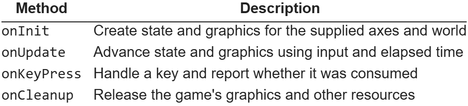
The launcher calls onUpdate on its active game, and MATLAB dispatches that call to the selected subclass. Pong implements paddle and ball movement; Flappy Bird advances its bird and pipes. All games inherit methods for scoring, combo handling and visual effects from GameBase. Window management, menus, timing and common services stay with the launcher.
As a handle class, GameBase lets the launcher keep a reference to the same game instance while its state changes. Position arrays, velocities, scores and graphics handles belong to that instance. Property access attributes allow the host to read the common score while leaving changes under the control of the game classes.
Flappy Bird creates its pipe patches in onInit, then reuses them throughout the game. Their handles and state are stored in private properties of the game instance. Its onUpdate method moves the active pipes across the playfield. Spawning a pipe selects an available pair, assigns its position and gap, and adds it to the active list. Once it leaves the playfield, the pair is hidden and its slot becomes available again:

In the default gravity-and-flap mode, the onKeyPress input handler sets a pending flap flag. The next update applies the upward impulse and clears the flag.
When the window closes, Arcade stops and deletes its timer, calls the active game's onCleanup method and clears its effects before deleting the figure. The smaller examples use MATLAB's onCleanup object to delete their own figure when the function exits. The requestClose callback function assigned to the figure’s CloseRequestFcn property sets a stop flag, letting the current update finish before cleanup removes the graphics.
Recent work on MATLAB graphics and performance
The MathWorks graphics team has also been improving the underlying rendering system. Maddie Moon's article about WebGL describes the R2025a transition, which brought the renderer already used by uifigure to regular MATLAB figures, along with work on stability, consistency and smoothing. Will Jackson also explains related changes to built-in panning, zooming and rotation in his article on the new interactions system.
R2025b focused on quality and stability improvements, building on the changes introduced in R2025a. It also improved performance when capturing successive frames in a loop with getframe, the function used by Arcade’s recording helper to capture and store frames for GIFs and videos.
R2026a included memory and stability improvements for graphics such as scatter and surface plots, described in Adam Danz's overview and the release notes. In addition, Jessa Karlberg describes the redesigned axes toolbar in R2026a, which allows seamless hovering without the animation slowdown issues caused by the toolbar’s continuous mouse tracking in earlier releases, eliminating the need to remove the toolbar as a workaround.
R2026b improved responsiveness for large data visualizations, with plot and plot3 being able to display lines and markers incrementally and shortening the wait time for the first visible results. MathWorks also reports automatic selection of a dedicated rendering GPU on supported Windows and Linux systems with multiple GPUs. These changes are documented in the release notes and the GPU-selection update.
info = rendererinfo;
info.GraphicsRenderer
info.RendererDevice
Mike Croucher also describes a new object-management system for R2026b, which can speed up object-oriented MATLAB code by reducing the cost of creating and deleting objects, as well as accessing their properties. The system is currently available as a beta and can be enabled through a package on File Exchange. Its documentation explains the changes to object lifecycle and compatibility.
Developing MATLAB code with AI
Arcade was developed with Claude Code through the MATLAB MCP Server, and the contest welcomes AI assistance as an option.
When working with an AI assistant, consider sharing your project's requirements and any existing code it can build on. Arcade's developer guide, for example, describes the shared game interface and explains how to add a new game. For your own game, you could begin with the main interaction and add features gradually, playing and improving it as you go. When something goes wrong, describe what happened and how to reproduce the problem, such as a ball passing through a wall at higher speeds.
The MATLAB Agentic Toolkit provides workflows for code review, analysis and testing. Its setup guide covers connecting MATLAB to AI applications including Claude Code, GitHub Copilot, OpenAI Codex, Gemini CLI and Amp, and installing MATLAB-specific skills. Through the MCP server, the AI assistant can run MATLAB code and tests, inspect the results, and use them to help diagnose problems and revise the code.
Several implementation choices in Arcade align with the MATLAB Coding Guidelines and performance rules: using a handle class for an object whose identity persists, restricting access to its state, retaining graphics, preallocating known-size arrays and cleaning up timers. The two downloadable examples presented above were checked with MATLAB Code Analyzer and tested for resizing, input, handle reuse and cleanup.
I hope that this article gives you something to experiment with, and perhaps a starting point for the One-Button Game Mini Hack. I look forward to seeing what you make!

I wanted to just enter and see whats happening.Found some interesting games here.
And i didnt have much experience with matlab code and honestly AI is there to create, if i want a lil changes i could do it. SO i went to chatgpt, i asked it to give me some ideas, it gave me typical few ones , i picked a laser smthin game and asked it to create. My bad i didnt give it exactly what i want to happen in the game, i itself couldnt figure out how to play it so i just deleted the code.
I got inspired from a game from on of the events a few months ago and wanted to recreate it in matlab. Gave the idea to ai , told exactly how and what i want , It gave me.
SO the whole point is AI works if you know how to make it work.
I used AI to create my REACT RUSH game. Its basically tells u ur reaction time. You guys can check it out here:
https://in.mathworks.com/matlabcentral/communitycontests/contests/10/entries/16637

In Flip Break, the paddle moves on its own and turns around at the edges. You decide when to reverse it and when to boost it to triple speed. The goal is not just to catch the ball, but to meet it with the part of the paddle that sends it toward a surviving brick.

Play with two control schemes
On the title screen, NORMAL and SWAPPED alternate about every 1.5 seconds. Click or press Space to select the displayed scheme and start.
- NORMAL: The first press reverses the paddle. A second press within 0.24 s boosts it to 3× speed.
- SWAPPED: The first press boosts the paddle to 3× speed. A second press within 0.24 s cancels the boost and reverses the paddle.
The first press acts immediately. The second counts only if received in a later update, and it does not undo the movement from the first. Try both schemes on the same board: which action would you rather have on the first press?

Clear all 55 bricks to see Congratulations!. Press once to see Speed Up, then again to start the next round with the same controls. After n clears, both the paddle and ball use 1 + 0.05*n times their starting speeds: 100%, 105%, 110%, and so on. The double-tap window stays the same.
Aim with the point of contact
At a wall, the game reverses the velocity component perpendicular to it. At the paddle, it keeps the ball's speed but picks a direction from six preset angles. Try hitting just right of center (20° from vertical), then near the right edge (60°). Before the next collision, sideways travel divided by vertical rise is tan(θ). For the same rise, the 60° shot travels about 4.8 times as far sideways. The angles are game rules, not a physical model of a paddle.
Calculate what happens between frames
Rather than checking only the ball's end position, the game calculates when the moving circle first touches a brick's face or corner. It advances to the earliest event and then processes the rest of the update. The bounce follows a separate game rule: a brick corner reverses both velocity components. For the paddle, the game checks horizontal overlap when the bottom of the ball reaches the paddle's top, using the ball's horizontal velocity relative to the paddle. A boost can put the paddle under the ball just in time.
Implementation and testing
The collision and paddle-angle routines came from an earlier Breakout prototype. The Mini Hack version separates initialization, updates, and rendering, and reuses its graphics objects. Its single game.m passed the validator at 9,980 characters. The round test set up the last brick twice and let the game register each final hit. It checked both speeds at 105% and 110% and confirmed that a paddle bounce preserved ball speed. This was not a full manual playthrough.

I have been a loyal MATLAB user for 25 years, starting from my university days. While many of my peers migrated to Python, I stayed for the stability, compatibility, and clean environment. However, I am finding the 2025 version exceptionally laggy. Despite running it on an $10k high-end machine, simple tasks like viewing variables and plotting take up to 60 seconds - actions that were near instantaneous in the 2020 version. I want to stay continue with MATLAB, but this performance gap is a major hurdle and irritation. I hope these optimization issues can be addressed quickly.

So, I have a Calculus III midterm coming up. Naturally, instead of studying vector fields, I decided to make an entire game about them.
I'd call that studying, right?
After seeing that the MATLAB One-Button Game Mini Hack introduced a new STEM Education category, I immediately wanted to make something for it. Having spent the past few weeks learning about vector fields, divergence, curl, and line integrals, I figured this would be a fun way to put some of those concepts to use.
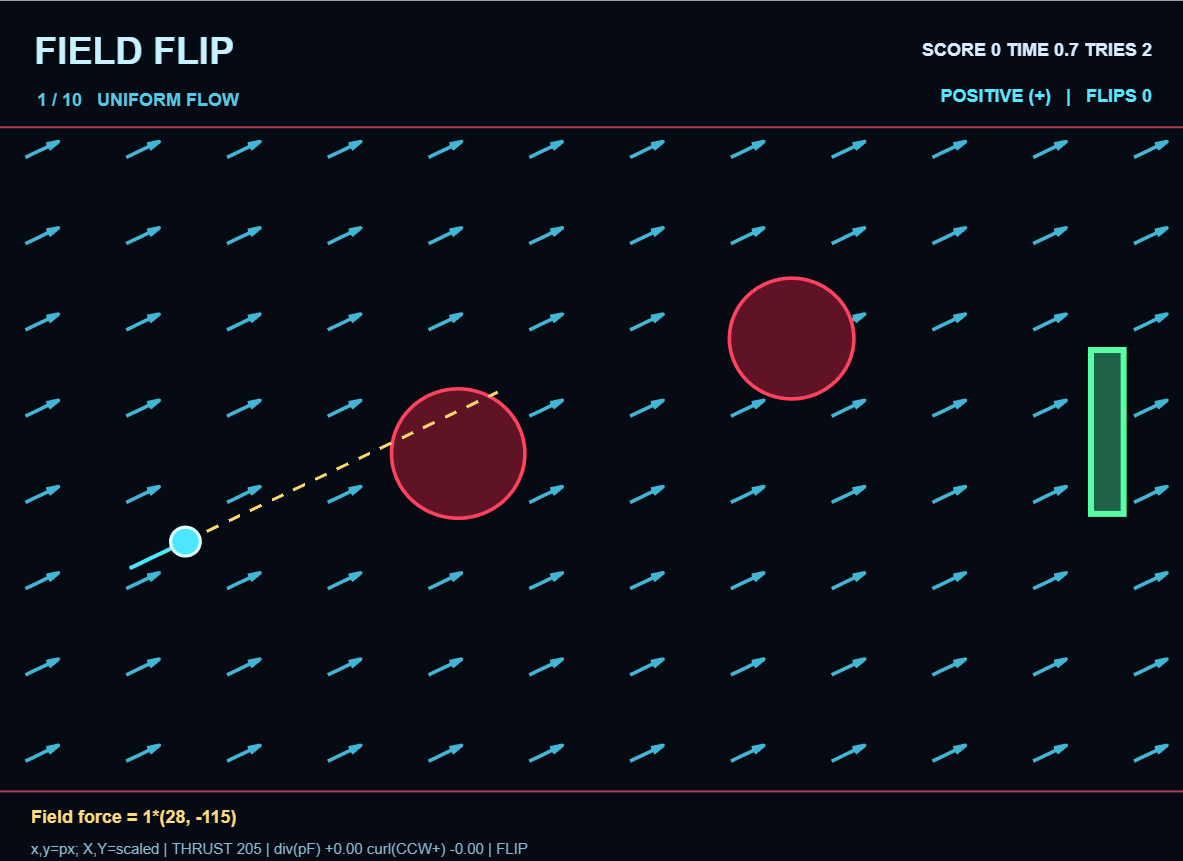
The idea is simple: you're a tiny particle navigating through a vector field, and your only ability is to reverse the direction of the field's force. Sounds easy enough, until you realize that Newton's laws of motion are not particularly interested in making your life easier.
With 10 increasingly challenging levels, you'll need to use momentum, polarity changes, and a little bit of vector calculus intuition to reach the exit.
How Do You Play?
You control a small particle traveling through a field of arrows. The arrows represent the combined force from the vector field and your particle's constant rightward thrust.
Your objective is to reach the green exit without crashing into any of the red obstacles or leaving the playable area.
There's just one button: SPACE (or click)!
- Your first tap starts the level.
- Every subsequent tap switches between positive and negative polarity.
- Positive polarity makes the field exert force in its original direction.
- Negative polarity reverses the field's force.
One thing to remember: flipping polarity doesn't instantly reverse your velocity!
Your particle has momentum. Even if the arrows suddenly point in the opposite direction, your particle might continue moving the same way until the opposing force slows it down.
Trust me, you'll become very familiar with this concept
The Yellow Line Is Your Best Friend!
You'll notice a dashed yellow line extending from your particle.
This is your predicted trajectory, calculated using the particle's current position, velocity, and forces.
It predicts approximately 1.7 seconds of movement, assuming you don't flip polarity again.
Rather than just hoping your particle avoids an obstacle, use this line to see where you're heading.
Pro tip: If the yellow line is heading straight into a giant red circle, you might want to, you know, press SPACE.
Don't Follow The Arrows Blindly!
The arrows show the direction of the current applied force, including thrust, but that doesn't necessarily mean your particle is moving in that direction.
Remember Newton's Second Law?
F = ma
Force changes acceleration, which changes velocity, which eventually changes position.
This means you need to anticipate where your particle will go rather than simply react to where it currently is.
A well-timed polarity flip can slow your particle down, redirect it, or help it narrowly avoid a collision.
A poorly timed flip can send it directly into an obstacle.
I have extensive experience with the second option.
The equation for the current field appears at the bottom of the screen, along with its divergence and curl.
You don't need to solve any integrals to beat the game, but understanding how the fields behave can make navigating them significantly easier.
Who knew Calculus III could actually be useful?
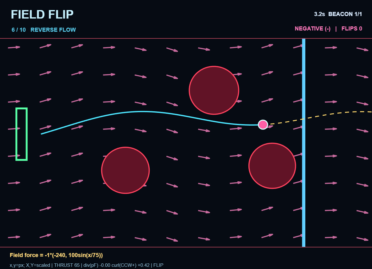
Things Get Interesting After Level 5
Your particle now has less rightward thrust, making it possible for the vector field to push you backward.
You'll also encounter beacons that must be collected before the exit unlocks.
Level 6 introduces the mechanic with one beacon. Levels 7–10 take things further, requiring you to travel back and forth across the field to collect three sequential beacons before returning to the exit on the left.
Yes, that means going through the obstacles multiple times.
And no, the obstacles do not become any friendlier on your second visit.
Some Final Advice
If there's one thing I hope players take away from FIELD FLIP, it's that a vector field describes how forces behave throughout space, but understanding motion requires considering velocity and acceleration too.
The particle doesn't magically follow whichever direction an arrow points. Its movement is the result of forces acting over time.
That distinction is what makes the gameplay interesting, and it's also one of the reasons I wanted to build the game in the first place.
Hopefully, FIELD FLIP makes vector fields a little more intuitive for anyone learning vector calculus, physics, or engineering.
And hopefully, creating it has somehow prepared me for my Calculus III midterm.
If not, at least I have a game to show for it.
Good luck, have fun, and try not to become too personally acquainted with the red circles...
Let me know what level you make it to, and whether you manage to beat all ten!

I have submitted a Quantum Mechanics inspired game named "Quantum Collapse!" to celebrate the STEM week of the OBGMH contest.
The rest of this post can be read in the comment below as I seem to be unable to submit text with LaTeX code and/or multiple hyperlinks.

Can a single button create order from chaos?
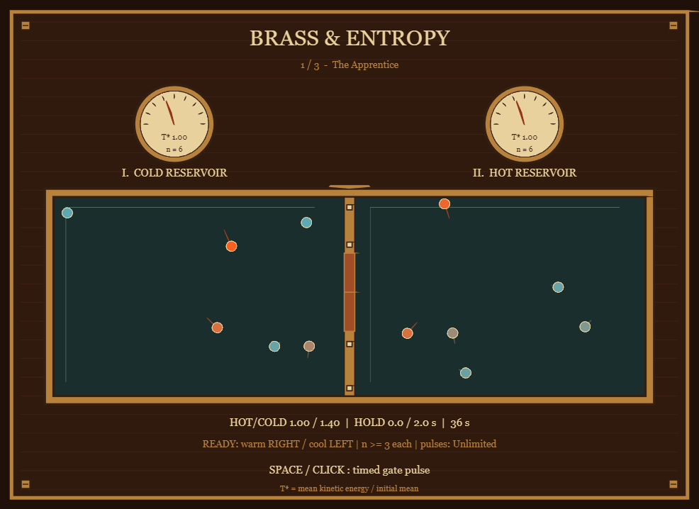
BRASS & ENTROPY is an educational puzzle game inspired by Maxwell's demon. The goal is to create a temperature difference between two gas chambers by controlling a mechanical gate.
The game combines particle dynamics, thermodynamics and a Victorian visual aesthetic, entirely within MATLAB.
1. Turning physics into gameplay
Twelve particles move continuously through two chambers. Each button press temporarily opens the gate, allowing particles to move between them.
The player must guide faster particles toward the hot chamber and slower particles toward the cold chamber.
Across three experiments, the required temperature ratio increases, while population constraints and a limited number of gate openings make the final challenge more demanding.
2. Simulating elastic collisions
Particle collisions are calculated using the relative velocity projected onto the collision normal.
For two particles of equal mass:
nv=dv/dist;
vn=sum((s.v(i,:)-s.v(j,:)).*nv);
if vn<0
s.v(i,:)=s.v(i,:)-vn*nv;
s.v(j,:)=s.v(j,:)+vn*nv;
end
The condition vn<0 ensures that the velocity correction is applied only when the particles are approaching each other.
This preserves kinetic energy and momentum during particle-particle collisions.
3. Calculating relative temperature
Rather than assigning an arbitrary temperature to each chamber, the simulation calculates a relative temperature from the mean kinetic energy of its particles:
e=sum(s.v.^2,2)/2;
left=s.p(:,1)<400;
s.N=[sum(left) sum(~left)];
s.T=[sum(e(left)) sum(e(~left))]./max(s.N,1)/s.e0;
s.R=s.T(2)/max(s.T(1),1e-10);
Logical indexing and vectorized operations allow both chambers to be evaluated efficiently.
The temperature indicators therefore respond directly to the simulated particle dynamics.
4. Improving simulation stability
To reduce missed collisions, each frame is divided into smaller physics steps:
n=ceil(dt/.003);
h=dt/n;
This limits each simulation step to approximately 3 milliseconds, independently of the rendering frame rate.
During prototype testing, the maximum relative energy error was approximately 1.78 × 10⁻¹⁵.
5. Creating a Victorian laboratory
All visual elements are generated procedurally in MATLAB, including brass frames, glass chambers, particle trails, analog temperature gauges and the animated mechanical gate.
Graphics objects are created during initialization and reused throughout gameplay, avoiding unnecessary object creation.
6. What the experiment teaches
The game illustrates how selective particle transport can create a difference in mean kinetic energy.
It is an idealized model of Maxwell's demon. Information processing and memory-erasure costs are not included, so the simulation does not imply a violation of the second law of thermodynamics.
Developed using OpenAI Codex and MATLAB MCP, the game was manually playtested, numerically verified and successfully validated within the 10,000-character limit.
Play BRASS & ENTROPY:

Hello everyone, I hope you all had a fantastic MATLAB EXPO! I wanted to create a forum for people to ask follow-up questions or start discussions related to the workshop Hands-On Agentic AI for Engineered Systems with MATLAB and Simulink. We ran this workshop nine (!) times over the two days of MATLAB EXPO, and heard some incredibly insightful comments and questions in each session, so I wanted to make a central bulletin board for people to share their thoughts and hear insights. A few ideas:
- What did you most enjoy about the workshop?
- Are there any topics/exercises that weren't clear, or maybe an area you want to explore more?
- Do you have an idea for how you'd like to apply agentic AI in your work?
MATLAB EXPO may be over, but that doesn't mean the conversation has to end!
In week 2, we are excited to see that the overall quality of entries went up. The games became more polished, creative, and ambitious.
Week 1: We were supposed to pick 5 winners. We picked 12.
Week 2: We tried to be more selective. We picked 13!
We’re especially excited about our new STEM Education category. This week we selected 6 winning entries, spanning topics including physics, biology, health, and engineering:
- Soobok / TRANSCRIPTION - one-button climber
- Roatis / RESONANCE — Master the Frequency
- Ahmed / Beat the PID
- Raffaele / X-Ray Guided: a coronary stenting simulator on one fluoro pedal
- Jan Studnicka / Pacemaker
- Shuen / Orbital Rendezvous
This is exactly what we hoped to see: learning through play. And remember, STEM Education comes with a special prize: a MathWorks Stainless Steel Coffee Mug! ☕
The category continues through Week 3, so keep the STEM games coming!
Week 2 Winners for other categories. Congratulations!
Visualization:
Humor:
Physics-Inspired
Game Design:

Earlier this year a bunch of MATLAB users got together to talk about their hobbies in a lightning talk format.
- Using "UIHTML" to create app components and Lightning
- Creating generative art with MATLAB
- Making MATLAB run on the Steam Deck (it was a wager)
Do you use MATLAB for hobbies?
I submitted a game called Sticky 8 last week inspired by a puzzle from Quanta Magazine. The puzzle is about understanding entropy in a toy universe, whereas my game is just about letting a figure 8 remain unlit (in that puzzle's terminology, keeping the entropy from reaching its minimum). It is made with help from an AI agent (the free one showcased in this starter article). Since this game did not fit in any of the familiar game categories, the AI asked quite a few questions regarding what I meant by bars sticking on a 7-segment display, what was to be scored, what was to be penalized, what kind of timings I was after, etc? After answering those questions as best as I could and half a dozen iterations trying to fix the "timings" & "characters limit" issues, a more or less working version was ready. I tweaked this last version a lot myself to bring the character count down to "4999" as I ran out of agent's "free time" for the day! 😂
Anyway, two interesting things I learnt from the agent (the first was done by the agent on its own while the second was suggested by me):
- Input Guard: Retain a screen for a bit longer by ignoring accidental button/space presses like after a round's result is displayed. For this purpose set a state variable "S.gd=0.6;" (for 0.6s delay) as the result screen loads. Let that variable decrease by "dt" in the updateState() function: "S.gd=S.gd-dt;". And before the next round loads, check not just for "pressed" state but also "S.gd<=0". Bingo! Your game player is not frustated by their best score vanish right before their eyes.🥳
- Title Fly-out: This powerpoint-style transition effect was quite easily implemented (by the agent). Here's the problem description: the title on the title screen is to be animated from its prominent screen position to the top of the screen, while its fontsize decreases and its colour fades to white. The following code loops inside the "renderFrame()" function (with the initialization code setting "S.anT=s.t;" and "S.t" increasing with "dt" somewhere in the "updateState()" function):
p = min(max((S.t - S.anT)/.9, 0), 1); %0.9s is the time duration for the animation
pe = p^2 * (3 - 2*p); % smooth-step easing!?
set(G.titleH, Position=[2.5,3.5+.591*pe], FontSize=38-22*pe, Color=cg+([1 1 1]-cg)*pe);
%So the header title's Position(2) changes from 3.5 to 4.091; Fontsize changes
%from 38 to 16; Color changes from cg=[1 0 1] to [1 1 1]=w smoothly!

That's all for now. Enjoy!🎉

My One-Button Game Mini Hack entry, HOT AIR PILOT, is a hot-air balloon game with a single control. A tap fires the burner. The balloon rises while the air inside is hot, sinks as it cools, and drifts with whichever wind layer it is in. The goal is to land on a green field a couple of kilometers away.
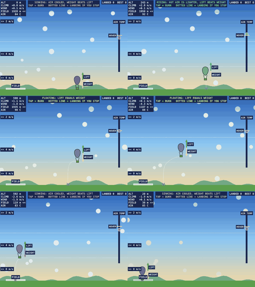
The physics in a few lines
A balloon floats when the hot air inside it is lighter than the air outside. At the same pressure, density goes as one over absolute temperature, so the lift is
ri = r * To / T; % density of the hot air inside
lift = (r - ri) * V * 9.81; % upward force from the hot air
The game compares that lift with the weight of the envelope, basket and pilot, and applies drag. Heat leaks out with Newton's law of cooling, so the inside temperature relaxes toward the outside temperature. A burn adds 3 K. The result feels like holding a ball up with short pushes, because every burn fades away within a few seconds.Putting the lesson on the screen
Two gauges show the balance directly. A green arrow shows the lift and a red arrow shows the weight, and the text at the top reads RISING, FLOATING or SINKING depending on which is larger. On the right, a thermometer shows the inside temperature as a dot and the temperature needed to float as a yellow tick. Solving lift equals weight for the temperature gives the tick:
T = (288.15 - .0065*z) / (1 - M / (rho(z)*V));
As the balloon climbs the air gets thinner, so the tick moves up. Players learn to chase the tick with taps before anyone tells them why.
A forecast made from the same step function
The dotted line is the part players like most. It is the balloon's own update function run forward in 6-second steps with no more burns, until it touches the ground:
for k = 1:300
[x,z,vx,vz,T] = stp(S,x,z,vx,vz,T,6);
S.fx(k) = x; S.fz(k) = max(z,0);
if z <= 0, break; end
end
One function, stp, does both the real flight and the forecast, so the line is always consistent with the game. It bends where the wind changes and it slides sideways each time the player burns, which is wind shear and thermal lag drawn in one picture.
Moving clouds as a wind display
Wind layers need to be visible without a chart. Sixteen clouds are a single scatter object. Each cloud has its own altitude, and each frame its x position moves by the wind at that altitude:
S.cx = mod(S.cx + wnd(S,(S.cy-40)/.24)*12*dt + 50,900) - 50;
Because wnd accepts a vector, no loop is needed. Clouds in different layers slide in different directions, and a player sees the shear before reading a number.
Tuning with a script pilot
My first version let the balloon hover for many seconds after the last burn, and the landing point swung by hundreds of meters. I wrote a small pilot script that climbs, holds altitude and stops burning when the forecast reaches the field, and ran it over random flights. A shorter cooling time and smaller burns made the forecast steady enough to use. If your game has a skill a script can play, it is worth testing that the script can win at human reaction times.
Which wind layer did you end up using?

A one-button game where the hard part is deciding, not tapping.
Radioembolization treats liver tumours from the inside: millions of glass microspheres loaded with yttrium-90 are injected into the hepatic artery, and they stop wherever the blood takes them. There is no steering after the injection. The whole art is choosing where to inject: far enough downstream to spare healthy liver, but upstream of every branch that feeds the tumour. And sometimes the honest answer is: nowhere, do not treat.
That is a single decision made with a catheter tip that slides along an arterial tree, which felt like a natural fit for one button. I am a medical physicist working with X-ray imaging, and after my first entry (X-Ray Guided, coronary stenting) I wanted to try a game where the difficulty is clinical judgement rather than reflexes.
How to play
A shift is 6 patients, each with a different theme: a simple case, lesions in both lobes, a high lung shunt, a bulky tumour, cirrhosis with a poorly vascularised tumour, and a random mix. Anatomy, arteries and lesions are different every time.
- Angiography: the catheter tip runs back and forth along the hepatic arteries. Tap to mark an injection point (up to two), tap while the tip is in the aorta when you are done. Common or proper hepatic artery means the whole liver, a lobar trunk one lobe, a segmental branch only the part of the lobe it feeds. Each tumour is fed by the branch it grows on.
- MAA simulation: a scan shows what you really perfuse, in red. Is the whole tumour red? How much healthy liver? How much goes to the lungs? The activity is planned automatically and the bars show tumour, liver and lung doses against their limits. A menu cycles: approve, go back to the angio (new MAA, small penalty), or decline the patient.
- Report: the post-treatment Y-90 PET, then the 3-month follow-up: treated tumour gone, under-dosed or untreated tumour still there, harmed organs in red.
A complication, or declining a patient who could have been treated, costs a life. About one patient in six has no safe plan at all: spotting those is part of the game.
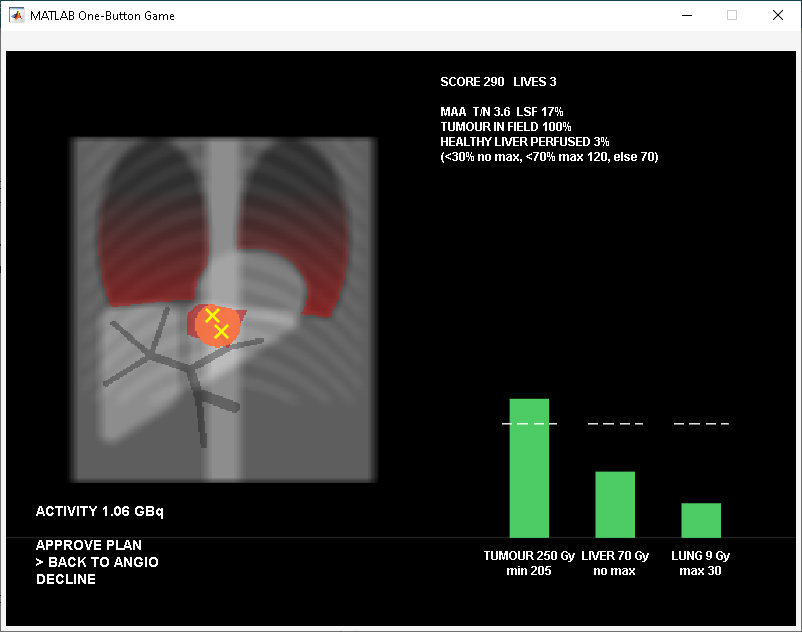
Real vs. playable
What I kept real
- The workflow: angiography, MAA simulation from the same catheter position, dosimetry, treatment, post-treatment imaging, follow-up.
- Dosimetry is the partition model used clinically: the activity in the perfused territory is shared between tumour and healthy liver in proportion to their masses and to the tumour-to-normal uptake ratio (T/N), and the lung gets the shunted fraction.
- Limits follow published recommendations for glass microspheres, simplified: tumour at least 205 Gy, lung at most 30 Gy, and a healthy-liver limit that depends on how much liver you irradiate (no limit for a small segmental treatment, 120 Gy for a lobe with enough liver spared, 70 Gy for most of the liver, lower with cirrhosis).
- The MAA is only a predictor: the T/N of the spheres can differ from the MAA, so the plan aims at 250 Gy to keep a margin.
- Clues are where they would be: a poorly vascularised tumour shows a faint blush on the angiogram, before the MAA confirms the low T/N.
What I changed for playability
- Synthetic anatomy: one projection, a liver cut into two lobes, 3 + 2 segmental branches, territories assigned to the nearest branch.
- At most two injection points. A tumour that would need three forces you upstream, at the cost of more healthy liver, which is exactly the trade-off I wanted to show.
- The catheter moves by itself, at constant speed: the tap is a choice, not a reflex test.
- The activity is computed for you, and the infusion itself is skipped: in real life the critical decision is the position, and that is what you play.
Three things I learned
1. A one-button game can be a game of decisions. If the game moves things by itself, when you tap becomes the input, and a cycling menu turns one button into any number of choices. Show what the tap does right now, and keep the cycle slow enough to read:
o = mod(floor((t-3)/1.5),3); % 0 approve, 1 back to angio, 2 decline
2. Hidden rules must become visible, or they feel unfair. My first versions had invisible random weights on the vascular territories and lesions placed anywhere: a tumour that clearly sat on one branch could end up 87 % covered, and nobody understood why. Now territories are simply “nearest branch”, every number that decides the outcome is on screen, and the report says why things went wrong. The game became harder to win and much easier to accept.
3. Vectorised geometry is cheap in characters. Territories, coverage and doses are a few array operations on a 256x256 grid, with no loops over pixels:
[~,i] = min(D,[],3); % D(:,:,k): distance from branch k
s.Tm = i==reshape(1:7,1,1,7) & s.v; % one logical map per territory
k = 49.67*A*(1-L)/(tn*s.q+s.w); % partition model: dose to healthy liver
What would you treat, and what would you decline? And if you work in interventional radiology or nuclear medicine: what did I oversimplify?
About Discussions
Discussions is a user-focused forum for the conversations that happen outside of any particular product or project.
Get to know your peers while sharing all the tricks you've learned, ideas you've had, or even your latest vacation photos. Discussions is where MATLAB users connect!
Get to know your peers while sharing all the tricks you've learned, ideas you've had, or even your latest vacation photos. Discussions is where MATLAB users connect!
More Community Areas

MATLAB Answers
Ask & Answer questions about MATLAB & Simulink!

File Exchange
Download or contribute user-submitted code!

Cody
Solve problem groups, learn MATLAB & earn badges!

Blogs
Get the inside view on MATLAB and Simulink!

AI Chat Playground
Use AI to generate initial draft MATLAB code, and answer questions!

