View Network Behavior Using tsne

This example shows how to use the tsne function to view activations in a trained network. This view can help you understand how a network works.

The tsne (Statistics and Machine Learning Toolbox) function in Statistics and Machine Learning Toolbox™ implements t-distributed stochastic neighbor embedding (t-SNE) [1]. This technique maps high-dimensional data (such as network activations in a layer) to two dimensions. The technique uses a nonlinear map that attempts to preserve distances. By using t-SNE to visualize the network activations, you can gain an understanding of how the network responds.

You can use t-SNE to visualize how deep learning networks change the representation of input data as it passes through the network layers. You can also use t-SNE to find issues with the input data and to understand which observations the network classifies incorrectly.

For example, t-SNE can reduce the multidimensional activations of a softmax layer to a 2-D representation with a similar structure. Tight clusters in the resulting t-SNE plot correspond to classes that the network usually classifies correctly. The visualization allows you to find points that appear in the wrong cluster, indicating an observation that the network classifies incorrectly. The observation might be labeled incorrectly, or the network might predict that an observation is an instance of a different class because it appears similar to other observations from that class. Note that the t-SNE reduction of the softmax activations uses only those activations, not the underlying observations.

Download Data Set

This example uses the Example Food Images data set, which contains 978 photographs of food in nine classes and is approximately 77 MB in size. Download the data set into your temporary directory by calling the downloadExampleFoodImagesData helper function; the code for this helper function appears at the end of this example.

dataDir = fullfile(tempdir, "ExampleFoodImageDataset");
url = "https://www.mathworks.com/supportfiles/nnet/data/ExampleFoodImageDataset.zip";

if ~exist(dataDir, "dir")
    mkdir(dataDir);
end

downloadExampleFoodImagesData(url,dataDir);

Downloading MathWorks Example Food Image dataset...
This can take several minutes to download...
Download finished...
Unzipping file...
Unzipping finished...
Done.

Train Network to Classify Food Images

Modify the SqueezeNet pretrained network to classify images of food from the data set. Replace the final convolutional layer, which has 1000 filters for the 1000 classes of ImageNet, with a new convolutional layer that has only nine filters. Each filter corresponds to a single type of food.

lgraph = layerGraph(squeezenet());
lgraph = lgraph.replaceLayer("ClassificationLayer_predictions",...
    classificationLayer("Name", "ClassificationLayer_predictions"));

newConv =  convolution2dLayer([14 14], 9, "Name", "conv", "Padding", "same");
lgraph = lgraph.replaceLayer("conv10", newConv);

Create an imageDatastore containing paths to the image data. Split the datastore into training and validation sets, using 65% of the data for training and the rest for validation. Because the data set is fairly small, overfitting is a significant issue. To minimize overfitting, augment the training set with random flips and scaling.

imds = imageDatastore(dataDir, ...
    "IncludeSubfolders", true, "LabelSource", "foldernames");

aug = imageDataAugmenter("RandXReflection", true, ...
    "RandYReflection", true, ...
    "RandXScale", [0.8 1.2], ...
    "RandYScale", [0.8 1.2]);

trainingFraction = 0.65;
[trainImds,valImds] = splitEachLabel(imds, trainingFraction);

augImdsTrain = augmentedImageDatastore([227 227], trainImds, ...
    'DataAugmentation', aug);
augImdsVal = augmentedImageDatastore([227 227], valImds);

Create training options and train the network. SqueezeNet is a small network that is quick to train. You can train on a GPU or a CPU; this example trains on a CPU.

opts = trainingOptions("adam", ...
    "InitialLearnRate", 1e-4, ...
    "MaxEpochs", 30, ...
    "ValidationData", augImdsVal, ...
    "Verbose", false,...
    "Plots", "training-progress", ...
    "ExecutionEnvironment","cpu",...
    "MiniBatchSize",128);
rng default
net = trainNetwork(augImdsTrain, lgraph, opts);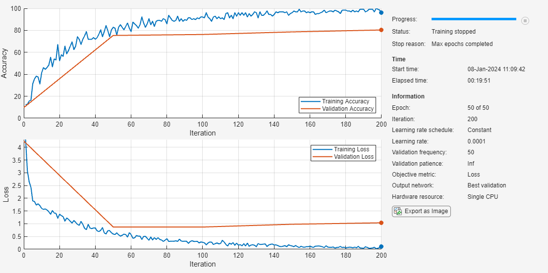

Classify Validation Data

Use the network to classify images in the validation set. To verify that the network is reasonably accurate at classifying new data, plot a confusion matrix of the true and predicted labels.

figure();
YPred = classify(net,augImdsVal);
confusionchart(valImds.Labels,YPred,'ColumnSummary',"column-normalized")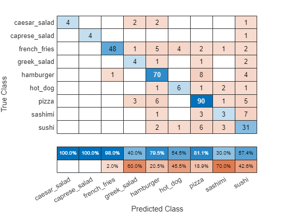

The network classifies several images well. The network appears to have trouble with sushi images, classifying many as sushi but some as pizza or hamburger. The network does not classify any images into the hot dog class.

Compute Activations for Several Layers

To continue to analyze the network performance, compute activations for every observation in the data set at an early max pooling layer, the final convolutional layer, and the final softmax layer. Output the activations as an NxM matrix, where N is the number of observations and M is the number of dimensions of the activation. M is the product of spatial and channel dimensions. Each row is an observation, and each column is a dimension. At the softmax layer M = 9, because the food data set has nine classes. Each row in the matrix contains nine elements, corresponding to the probabilities that an observation belongs to each of the nine classes of food.

earlyLayerName = "pool1";
finalConvLayerName = "conv";
softmaxLayerName = "prob";
pool1Activations = activations(net,...
    augImdsVal,earlyLayerName,"OutputAs","rows");
finalConvActivations = activations(net,...
    augImdsVal,finalConvLayerName,"OutputAs","rows");
softmaxActivations = activations(net,...
    augImdsVal,softmaxLayerName,"OutputAs","rows");

Ambiguity of Classifications

You can use the softmax activations to calculate the image classifications that are most likely to be incorrect. Define the ambiguity of a classification as the ratio of the second-largest probability to the largest probability. The ambiguity of a classification is between zero (nearly certain classification) and 1 (nearly as likely to be classified to the most likely class as the second class). An ambiguity of near 1 means the network is unsure of the class in which a particular image belongs. This uncertainty might be caused by two classes whose observations appear so similar to the network that it cannot learn the differences between them. Or, a high ambiguity can occur because a particular observation contains elements of more than one class, so the network cannot decide which classification is correct. Note that low ambiguity does not necessarily imply correct classification; even if the network has a high probability for a class, the classification can still be incorrect.

[R,RI] = maxk(softmaxActivations,2,2);
ambiguity = R(:,2)./R(:,1);

Find the most ambiguous images.

[ambiguity,ambiguityIdx] = sort(ambiguity,"descend");

View the most probable classes of the ambiguous images and the true classes.

classList = unique(valImds.Labels);
top10Idx = ambiguityIdx(1:10);
top10Ambiguity = ambiguity(1:10);
mostLikely = classList(RI(ambiguityIdx,1));
secondLikely = classList(RI(ambiguityIdx,2));
table(top10Idx,top10Ambiguity,mostLikely(1:10),secondLikely(1:10),valImds.Labels(ambiguityIdx(1:10)),...
    'VariableNames',["Image #","Ambiguity","Likeliest","Second","True Class"])

ans=10×5 table
    Image #    Ambiguity    Likeliest       Second        True Class 
    _______    _________    _________    ____________    ____________

       94        0.9879     hamburger    pizza           hamburger   
      175       0.96311     hamburger    french_fries    hot_dog     
      179       0.94939     pizza        hamburger       hot_dog     
      337       0.93426     sushi        sashimi         sushi       
      256       0.92972     sushi        pizza           pizza       
      297       0.91776     sushi        sashimi         sashimi     
      283       0.80407     pizza        sushi           pizza       
       27       0.80278     hamburger    pizza           french_fries
      302       0.79283     sashimi      sushi           sushi       
      201       0.76034     pizza        greek_salad     pizza       

The network predicts that image 27 is most likely hamburger or pizza. However, this image is actually French fries. View the image to see why this misclassification might occur.

v = 27;
figure();
imshow(valImds.Files{v});
title(sprintf("Observation: %i\n" + ...
    "Actual: %s. Predicted: %s", v, ...
    string(valImds.Labels(v)), string(YPred(v))), ...
    'Interpreter', 'none');

The image contains several distinct regions, some of which might confuse the network.

Compute 2-D Representations of Data Using t-SNE

Calculate a low-dimensional representation of the network data for an early max pooling layer, the final convolutional layer, and the final softmax layer. Use the tsne function to reduce the dimensionality of the activation data from M to 2. The larger the dimensionality of the activations, the longer the t-SNE computation takes. Therefore, computation for the early max pooling layer, where activations have 200,704 dimensions, takes longer than for the final softmax layer. Set the random seed for reproducibility of the t-SNE result.

rng default
pool1tsne = tsne(pool1Activations);
finalConvtsne = tsne(finalConvActivations);
softmaxtsne = tsne(softmaxActivations);

Compare Network Behavior for Early and Later Layers

The t-SNE technique tries to preserve distances so that points near each other in the high-dimensional representation are also near each other in the low-dimensional representation. As shown in the confusion matrix, the network is effective at classifying into different classes. Therefore, images that are semantically similar (or of the same type), such as caesar salad and caprese salad, are near each other in the softmax activations space. t-SNE captures this proximity in a 2-D representation that is easier to understand and plot than the nine-dimensional softmax scores.

Early layers tend to operate on low-level features such as edges and colors. Deeper layers have learned high-level features with more semantic meaning, such as the difference between a pizza and a hot dog. Therefore, activations from early layers do not show any clustering by class. Two images that are similar pixelwise (for example, they both contain a lot of green pixels) are near each other in the high-dimensional space of the activations, regardless of their semantic contents. Activations from later layers tend to cluster points from the same class together. This behavior is most pronounced at the softmax layer and is preserved in the two-dimensional t-SNE representation.

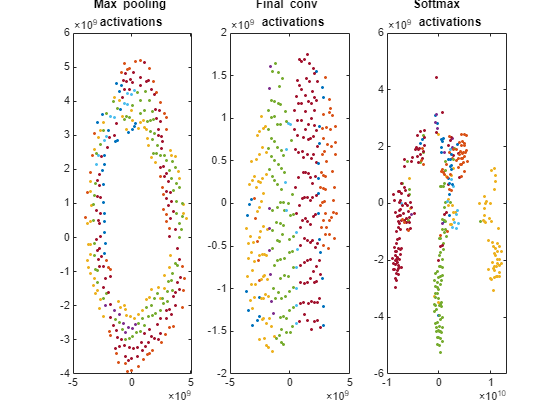
Plot the t-SNE data for the early max pooling layer, the final convolutional layer, and the final softmax layer using the gscatter function. Observe that the early max pooling activations do not exhibit any clustering between images of the same class. Activations of the final convolutional layer are clustered by class to some extent, but less so than the softmax activations. Different colors correspond to observations of different classes.

doLegend = 'off';
markerSize = 7;
figure;

subplot(1,3,1);
gscatter(pool1tsne(:,1),pool1tsne(:,2),valImds.Labels, ...
    [],'.',markerSize,doLegend);
title("Max pooling activations");

subplot(1,3,2);
gscatter(finalConvtsne(:,1),finalConvtsne(:,2),valImds.Labels, ...
    [],'.',markerSize,doLegend);
title("Final conv activations");

subplot(1,3,3);
gscatter(softmaxtsne(:,1),softmaxtsne(:,2),valImds.Labels, ...
    [],'.',markerSize,doLegend);
title("Softmax activations");

Explore Observations in t-SNE Plot

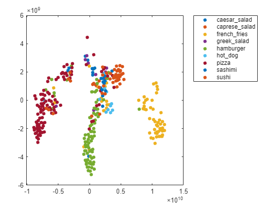
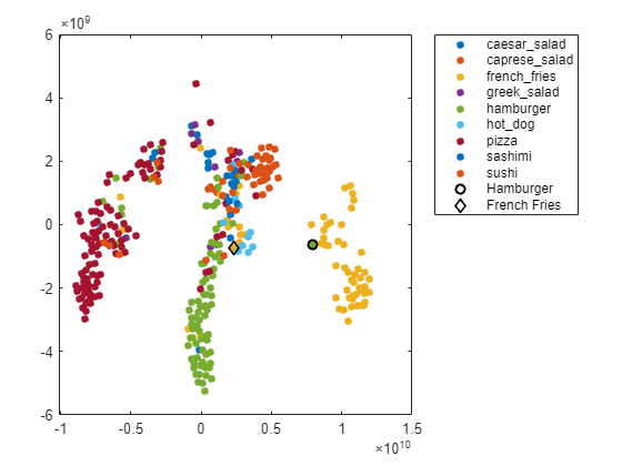
Create a larger plot of the softmax activations, including a legend labeling each class. From the t-SNE plot, you can understand more about the structure of the posterior probability distribution.

For example, the plot shows a distinct, separate cluster of French fries observations, whereas the sashimi and sushi clusters are not resolved very well. Similar to the confusion matrix, the plot suggests that the network is more accurate at predicting into the French fries class.

numClasses = length(classList);
colors = lines(numClasses);
h = figure;
gscatter(softmaxtsne(:,1),softmaxtsne(:,2),valImds.Labels,colors);

l = legend;
l.Interpreter = "none";
l.Location = "bestoutside";

You can also use t-SNE to determine which images are misclassified by the network and why. Incorrect observations are often isolated points of the wrong color for their surrounding cluster. For example, a misclassified image of hamburger is very near the French fries region (the green dot nearest the center of the orange cluster). This dot is observation 99. Circle this observation on the t-SNE plot, and display the image with imshow.

obs = 99;
figure(h)
hold on;
hs = scatter(softmaxtsne(obs, 1), softmaxtsne(obs, 2), ...
    'black','LineWidth',1.5);
l.String{end} = 'Hamburger';
hold off;
figure();
imshow(valImds.Files{obs});
title(sprintf("Observation: %i\n" + ...
    "Actual: %s. Predicted: %s", obs, ...
    string(valImds.Labels(obs)), string(YPred(obs))), ...
    'Interpreter', 'none');

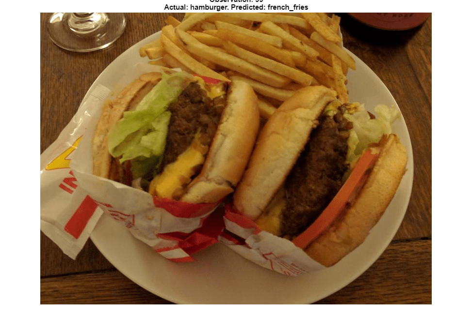
If an image contains multiple types of food, the network can get confused. In this case, the network classifies the image as French fries even though the food in the foreground is hamburger. The French fries visible at the edge of the image cause the confusion.

Similarly, the ambiguous image 27 (shown earlier in the example) has multiple regions. Examine the t-SNE plot highlighting the ambiguous aspect of this French fries image.

obs = 27;
figure(h)
hold on;
h = scatter(softmaxtsne(obs, 1), softmaxtsne(obs, 2), ...
    'k','d','LineWidth',1.5);
l.String{end} = 'French Fries';
hold off;

The image is not in a well-defined cluster in the plot, which indicates that the classification is likely incorrect. The image is far from the French fries cluster, and close to the hamburger cluster.

The why of a misclassification must be provided by other information, typically a hypothesis based on the contents of the image. You can then test the hypothesis using other data, or using tools that indicate which spatial regions of an image are important to network classification. For examples, see occlusionSensitivity and Grad-CAM Reveals the Why Behind Deep Learning Decisions.

References

[1] van der Maaten, Laurens, and Geoffrey Hinton. "Visualizing Data using t-SNE." Journal of Machine Learning Research 9, 2008, pp. 2579–2605.

Helper Function

function downloadExampleFoodImagesData(url, dataDir)
% Download the Example Food Image data set, containing 978 images of
% different types of food split into 9 classes.

% Copyright 2019 The MathWorks, Inc.

fileName = "ExampleFoodImageDataset.zip";
fileFullPath = fullfile(dataDir, fileName);

% Download the .zip file into a temporary directory.
if ~exist(fileFullPath, "file")
    fprintf("Downloading MathWorks Example Food Image dataset...\n");
    fprintf("This can take several minutes to download...\n");
    websave(fileFullPath, url);
    fprintf("Download finished...\n");
else
    fprintf("Skipping download, file already exists...\n");
end

% Unzip the file.
%
% Check if the file has already been unzipped by checking for the presence
% of one of the class directories.
exampleFolderFullPath = fullfile(dataDir, "pizza");
if ~exist(exampleFolderFullPath, "dir")
    fprintf("Unzipping file...\n");
    unzip(fileFullPath, dataDir);
    fprintf("Unzipping finished...\n");
else
    fprintf("Skipping unzipping, file already unzipped...\n");
end
fprintf("Done.\n");

end