Updated Discussions

While searching the internet for some books on ordinary differential equations, I came across a link that I believe is very useful for all math students and not only. If you are interested in ODEs, it's worth taking the time to study it.
A First Look at Ordinary Differential Equations by Timothy S. Judson is an excellent resource for anyone looking to understand ODEs better. Here's a brief overview of the main topics covered:
  1. Introduction to ODEs: Basic concepts, definitions, and initial differential equations.
  2. Methods of Solution:
  • Separable equations
  • First-order linear equations
  • Exact equations
  • Transcendental functions
  1. Applications of ODEs: Practical examples and applications in various scientific fields.
  2. Systems of ODEs: Analysis and solutions of systems of differential equations.
  3. Series and Numerical Methods: Use of series and numerical methods for solving ODEs.
This book provides a clear and comprehensive introduction to ODEs, making it suitable for students and new researchers in mathematics. If you're interested, you can explore the book in more detail here: A First Look at Ordinary Differential Equations.
goc3
goc3
Last activity on 7 Jun 2024

There are a host of problems on Cody that require manipulation of the digits of a number. Examples include summing the digits of a number, separating the number into its powers, and adding very large numbers together.
If you haven't come across this trick yet, you might want to write it down (or save it electronically):
digits = num2str(4207) - '0'
That code results in the following:
digits =
4 2 0 7
Now, summing the digits of the number is easy:
sum(digits)
ans =
13
The study of the dynamics of the discrete Klein - Gordon equation (DKG) with friction is given by the equation :
In the above equation, W describes the potential function:
to which every coupled unit adheres. In Eq. (1), the variable $$ is the unknown displacement of the oscillator occupying the n-th position of the lattice, and is the discretization parameter. We denote by h the distance between the oscillators of the lattice. The chain (DKG) contains linear damping with a damping coefficient , whileis the coefficient of the nonlinear cubic term.
For the DKG chain (1), we will consider the problem of initial-boundary values, with initial conditions
and Dirichlet boundary conditions at the boundary points and , that is,
Therefore, when necessary, we will use the short notation for the one-dimensional discrete Laplacian
Now we want to investigate numerically the dynamics of the system (1)-(2)-(3). Our first aim is to conduct a numerical study of the property of Dynamic Stability of the system, which directly depends on the existence and linear stability of the branches of equilibrium points.
For the discussion of numerical results, it is also important to emphasize the role of the parameter . By changing the time variable , we rewrite Eq. (1) in the form
. We consider spatially extended initial conditions of the form: where is the distance of the grid and is the amplitude of the initial condition
We also assume zero initial velocity:
the following graphs for and
% Parameters
L = 200; % Length of the system
K = 99; % Number of spatial points
j = 2; % Mode number
omega_d = 1; % Characteristic frequency
beta = 1; % Nonlinearity parameter
delta = 0.05; % Damping coefficient
% Spatial grid
h = L / (K + 1);
n = linspace(-L/2, L/2, K+2); % Spatial points
N = length(n);
omegaDScaled = h * omega_d;
deltaScaled = h * delta;
% Time parameters
dt = 1; % Time step
tmax = 3000; % Maximum time
tspan = 0:dt:tmax; % Time vector
% Values of amplitude 'a' to iterate over
a_values = [2, 1.95, 1.9, 1.85, 1.82]; % Modify this array as needed
% Differential equation solver function
function dYdt = odefun(~, Y, N, h, omegaDScaled, deltaScaled, beta)
U = Y(1:N);
Udot = Y(N+1:end);
Uddot = zeros(size(U));
% Laplacian (discrete second derivative)
for k = 2:N-1
Uddot(k) = (U(k+1) - 2 * U(k) + U(k-1)) ;
end
% System of equations
dUdt = Udot;
dUdotdt = Uddot - deltaScaled * Udot + omegaDScaled^2 * (U - beta * U.^3);
% Pack derivatives
dYdt = [dUdt; dUdotdt];
end
% Create a figure for subplots
figure;
% Initial plot
a_init = 2; % Example initial amplitude for the initial condition plot
U0_init = a_init * sin((j * pi * h * n) / L); % Initial displacement
U0_init(1) = 0; % Boundary condition at n = 0
U0_init(end) = 0; % Boundary condition at n = K+1
subplot(3, 2, 1);
plot(n, U0_init, 'r.-', 'LineWidth', 1.5, 'MarkerSize', 10); % Line and marker plot
xlabel('$x_n$', 'Interpreter', 'latex');
ylabel('$U_n$', 'Interpreter', 'latex');
title('$t=0$', 'Interpreter', 'latex');
set(gca, 'FontSize', 12, 'FontName', 'Times');
xlim([-L/2 L/2]);
ylim([-3 3]);
grid on;
% Loop through each value of 'a' and generate the plot
for i = 1:length(a_values)
a = a_values(i);
% Initial conditions
U0 = a * sin((j * pi * h * n) / L); % Initial displacement
U0(1) = 0; % Boundary condition at n = 0
U0(end) = 0; % Boundary condition at n = K+1
Udot0 = zeros(size(U0)); % Initial velocity
% Pack initial conditions
Y0 = [U0, Udot0];
% Solve ODE
opts = odeset('RelTol', 1e-5, 'AbsTol', 1e-6);
[t, Y] = ode45(@(t, Y) odefun(t, Y, N, h, omegaDScaled, deltaScaled, beta), tspan, Y0, opts);
% Extract solutions
U = Y(:, 1:N);
Udot = Y(:, N+1:end);
% Plot final displacement profile
subplot(3, 2, i+1);
plot(n, U(end,:), 'b.-', 'LineWidth', 1.5, 'MarkerSize', 10); % Line and marker plot
xlabel('$x_n$', 'Interpreter', 'latex');
ylabel('$U_n$', 'Interpreter', 'latex');
title(['$t=3000$, $a=', num2str(a), '$'], 'Interpreter', 'latex');
set(gca, 'FontSize', 12, 'FontName', 'Times');
xlim([-L/2 L/2]);
ylim([-2 2]);
grid on;
end
% Adjust layout
set(gcf, 'Position', [100, 100, 1200, 900]); % Adjust figure size as needed
Dynamics for the initial condition , , for , for different amplitude values. By reducing the amplitude values, we observe the convergence to equilibrium points of different branches from and the appearance of values for which the solution converges to a non-linear equilibrium point Parameters:
Detection of a stability threshold : For , the initial condition , , converges to a non-linear equilibrium point.
Characteristics for , with corresponding norm 
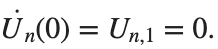
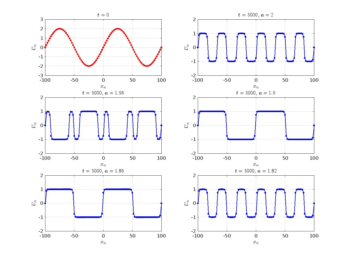
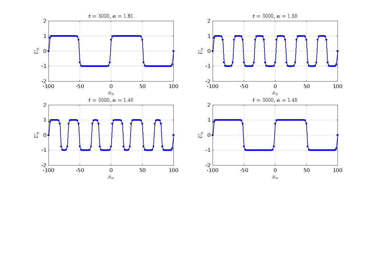
where the dynamics appear in the first image of the third row, we observe convergence to a non-linear equilibrium point of branch This has the same norm and the same energy as the previous case but the final state has a completely different profile. This result suggests secondary bifurcations have occurred in branch
By further reducing the amplitude, distinct values of are discerned: 1.9, 1.85, 1.81 for which the initial condition with norms respectively, converges to a non-linear equilibrium point of branch This equilibrium point has norm and energy . The behavior of this equilibrium is illustrated in the third row and in the first image of the third row of Figure 1, and also in the first image of the third row of Figure 2. For all the values between the aforementioned a, the initial condition converges to geometrically different non-linear states of branch as shown in the second image of the first row and the first image of the second row of Figure 2, for amplitudes and respectively.
Refference:
  1. Dynamics of nonlinear lattices: asymptotic behavior and study of the existence and stability of tracked oscillations-Vetas Konstantinos (2018)
Hans Scharler
Hans Scharler
Last activity on 31 May 2024

Spring is here in Natick and the tulips are blooming! While tulips appear only briefly here in Massachusetts, they provide a lot of bright and diverse colors and shapes. To celebrate this cheerful flower, here's some code to create your own tulip!
Dear members, I’m currently doing research on the subject of using Generative A.I. as a digital designer. What our research group would like to know is which ethical issues have a big impact on the decisions you guys and girls make using generative A.I.
Whether you’re using A.I. or not, we would really like to know your vision and opinion about this subject. Please empty your thoughts and oppinion into your answers, we would like to get as much information as possible.
Are you currently using A.I. when doing your job? Yes, what for. No (not yet), why not?
Using A.I., would you use real information or alter names/numbers to get an answer?
What information would or wouldn’t you use? If the client is asking/ordering you to do certain things that go against your principles, would you still do it because order is order? How far would you go?
Who is responsible for the outcome of the generated content, you or the client?
Would you still feel like a product owner if it was co-developed with A.I.?
What we are looking for is that we would like to know why people do or don’t use AI in the field of design and wich ethical considerations they make. We’re just looking for general moral line of people, for example: 70% of designers don’t feel owner of a design that is generated by AI but 95% feels owner when it is co-created.
So therefore the questions we asked, we want to know the how you feel about this.
Check out this episode about PIVLab: https://www.buzzsprout.com/2107763/15106425
Join the conversation with William Thielicke, the developer of PIVlab, as he shares insights into the world of particle image velocimetery (PIV) and its applications. Discover how PIV accurately measures fluid velocities, non invasively revolutionising research across the industries. Delve into the development journey of PI lab, including collaborations, key features and future advancements for aerodynamic studies, explore the advanced hardware setups camera technologies, and educational prospects offered by PIVlab, for enhanced fluid velocity measurements. If you are interested in the hardware he speaks of check out the company: Optolution.
One of the starter prompts is about rolling two six-sided dice and plot the results. As a hobby, I create my own board games. I was able to use the dice rolling prompt to show how a simple roll and move game would work. That was a great surprise!
How to leave feedback on a doc page
Leaving feedback is a two-step process. At the bottom of most pages in the MATLAB documentation is a star rating.
Start by selecting a star that best answers the question. After selecting a star rating, an edit box appears where you can offer specific feedback.
When you press "Submit" you'll see the confirmation dialog below. You cannot go back and edit your content, although you can refresh the page to go through that process again.
Tips on leaving feedback
  • Be productive. The reader should clearly understand what action you'd like to see, what was unclear, what you think needs work, or what areas were really helpful.
  • Positive feedback is also helpful. By nature, feedback often focuses on suggestions for changes but it also helps to know what was clear and what worked well.
  • Point to specific areas of the page. This helps the reader to narrow the focus of the page to the area described by your feedback.
What happens to that feedback?
Before working at MathWorks I often left feedback on documentation pages but I never knew what happens after that. One day in 2021 I shared my speculation on the process:
> That feedback is received by MathWorks Gnomes which are never seen nor heard but visit the MathWorks documentation team at night while they are sleeping and whisper selected suggestions into their ears to manipulate their dreams. Occassionally this causes them to wake up with a Eureka moment that leads to changes in the documentation.
I'd like to let you in on the secret which is much less fanciful. Feedback left in the star rating and edit box are collected and periodically reviewed by the doc writers who look for trends on highly trafficked pages and finer grain feedback on less visited pages. Your feedback is important and often results in improvements.
Hallo zusammen,
seit ein paar Tagen werden sämtliche meiner Visualisierungen nicht mehr aktualisiert. Im Editiermodus läuft der Code durch und die Grafik wird korrekt erzeugt.
Hat jemand eine Idee was da schief läuft?
Danke & viele Grüße
In the MATLAB description of the algorithm for Lyapunov exponents, I believe there is ambiguity and misuse.
The lambda(i) in the reference literature signifies the Lyapunov exponent of the entire phase space data after expanding by i time steps, but in the calculation formula provided in the MATLAB help documentation, Y_(i+K) represents the data point at the i-th point in the reconstructed data Y after K steps, and this calculation formula also does not match the calculation code given by MATLAB. I believe there should be some misguidance and misunderstanding here.
According to the symbol regulations in the algorithm description and the MATLAB code, I think the correct formula might be y(i) = 1/dt * 1/N * sum_j( log( ||Y_(j+i) - Y_(j*+i)|| ) )
Oleksandr
Oleksandr
Last activity on 28 May 2024

Let's talk about probability theory in Matlab.
Conditions of the problem - how many more letters do I need to write to the sales department to get an answer?
To get closer to the problem, I need to buy a license under a contract. Maybe sometimes there are responsible employees sitting here who will give me an answer.
Thank you
Ignacio
Ignacio
Last activity on 28 May 2024

I have an Arduino Uno R3 with an integrated ESP 8266. With the Arduino Uno, I measure some capacitive humidity sensors and a DHT 22 temperature and humidity sensor. The measurements are sent to the serial port and the ESP 8266 picks them up and uploads them to ThingSpeak. My problem is that it does this randomly and not in the assigned fields. Could someone help me? Thank you very much
Hello MATLAB Community!
We've had an exciting few weeks filled with insightful discussions, innovative tools, and engaging blog posts from our vibrant community. Here's a highlight of some noteworthy contributions that have sparked interest and inspired us all. Let's dive in!

Interesting Questions

Cindyawati explores the intriguing concept of interrupting continuous data in differential equations to study the effects of drug interventions in disease models. A thought-provoking question that bridges mathematics and medical research.
Pedro delves into the application of Linear Quadratic Regulator (LQR) for error dynamics and setpoint tracking, offering insights into control systems and their real-world implications.

Popular Discussions

Chen Lin shares an engaging interview with Zhaoxu Liu, shedding light on the creative processes behind some of the most innovative MATLAB contest entries of 2023. A must-read for anyone looking for inspiration!
Zhaoxu Liu, also known as slanderer, updates the community with the latest version of the MATLAB Plot Cheat Sheet. This resource is invaluable for anyone looking to enhance their data visualization skills.

From File Exchange

Giorgio introduces a toolbox for frequency estimation, making it simpler for users to import signals directly from the MATLAB workspace. A significant contribution for signal processing enthusiasts.

From the Blogs

Cleve Moler revisits a classic program for predicting future trends based on census data, offering a fascinating glimpse into the evolution of computational forecasting.
With contributions from Dinesh Kavalakuntla, Adam presents an insightful guide on improving app design workflows in MATLAB App Designer, focusing on component swapping and labeling.
We're incredibly proud of the diverse and innovative contributions our community members make every day. Each post, discussion, and tool not only enriches our knowledge but also inspires others to explore and create. Let's continue to support and learn from each other as we advance in our MATLAB journey.
Happy Coding!
We're thrilled to unveil a new feature in the MATLAB Central community: User Following.
Our community is so lucky to have many experienced MATLAB experts who generously share their knowledge and insights across different applications, including Answers, File Exchange, Discussions, Contests, or Blogs.
With the introduction of User Following feature, you can now easily track new content across different areas and engage in discussions with people you follow. Simply click the ‘Follow’ button located on their profile page to start.
Depending on your communication setting, you will receive notifications via email and/or view updates in your ‘Followed Activity’ feeds. To tailor your feed, select the ‘People’ filter and focus on activities from those you follow.
We strongly encourage you to take advantage of the User Following feature to foster learning and collaboration within our vibrant community.
Who will be the first person you choose to follow? Share your answer in the comments section below and let's inspire each other to explore new horizons together.
Cordial saludo , Necesito simular un generador electrico que tiene una entrada mecanica y genera el suficiente voltage y corriente para encender un LED.
Hassan Ali
Hassan Ali
Last activity on 25 May 2024

Hello everyone.
I have modelled a three phase inverter to run a 5Kw PMSM motor (MATLAB preparametrized). The torque load is applied through ideal torque source and step junction, and the speed of the motor is visualized. When I provide the gate signal only through SPWM generator (No control, only SPWM signal generation through carrier and sine wave comparison),
  • The speed stabilizes around 62 rad/sec after some initial oscillations, but when I try to run the same model using PMSM field oriented control block set, the speed is negative (negative rotation) and it keeps on increasing eventhough the speed reference provided is only upto 60. The waveform of both speed and torque has been attached hereby.
  • Moreover, is there anyway to tune the PI controllers (inner and outer loops) of PMSM Field oriented blockset automatically.
  • It can be seen from the torque waveform, there is soemkind of disturbance around 0.4-0.45 sec, which creates too much noise in current, torque waveforms. What could be the reason behind this.
Your help would be highly appreciated.
Thank you.
Jonny Pats
Jonny Pats
Last activity on 24 May 2024

Are you local to Boston?
Shape the Future of MATLAB: Join MathWorks' UX Night In-Person!
When: June 25th, 6 to 8 PM
Where: MathWorks Campus in Natick, MA
🌟 Calling All MATLAB Users! Here's your unique chance to influence the next wave of innovations in MATLAB and engineering software. MathWorks invites you to participate in our special after-hours usability studies. Dive deep into the latest MATLAB features, share your valuable feedback, and help us refine our solutions to better meet your needs.
🚀 This Opportunity Is Not to Be Missed:
  • Exclusive Hands-On Experience: Be among the first to explore new MATLAB features and capabilities.
  • Voice Your Expertise: Share your insights and suggestions directly with MathWorks developers.
  • Learn, Discover, and Grow: Expand your MATLAB knowledge and skills through firsthand experience with unreleased features.
  • Network Over Dinner: Enjoy a complimentary dinner with fellow MATLAB enthusiasts and the MathWorks team. It's a perfect opportunity to connect, share experiences, and network after work.
  • Earn Rewards: Participants will not only contribute to the advancement of MATLAB but will also be compensated for their time. Plus, enjoy special MathWorks swag as a token of our appreciation!
👉 Reserve Your Spot Now: Space is limited for these after-hours sessions. If you're passionate about MATLAB and eager to contribute to its development, we'd love to hear from you.
Hi Helpdesk,
I urgently seek assistance with an issue that has persisted for a week. I am using Node-RED to interface my gateway and vibration sensor. The sensor sends 960 packets of X, Y, and Z data every 5 minutes. I retrieve and send this data through my Thingspeak42 node to my Thingspeak channel.
I am subscribed to the Thingspeak Student paid plan (see attached "12.png"). Despite this, Thingspeak is inconsistently snipping my data. For example, my X-field sometimes receives only 78 out of 960 points, and similar inconsistencies occur with the Y and Z fields.
Attached is "vibration data node red.png," showing an attempt to send just 120 packets to my Thingspeak channel. However, only 93 data points are received. Also attached is a JSON snapshot of field 2 - X_values, showing only 93 points ("JSON Field 2 data.png"). This is disappointing given that I am paying for the student plan, which should support 33 million points/year per unit (~90,000/day per unit).
I urgently require an explanation and resolution for this issue. Please provide immediate assistance.
Kind regards,
Krish

Starting in r2020a, AppDesigner buttons and TreeNodes can display animated GIFs, SVG, and truecolor image arrays.

Every component in the App above is either a Button or a TreeNode!

Prior to r2020a the icon property of buttons and TreeNodes in AppDesigner supported JPEG, PNG, or GIF image files specified by a character vector or string array but did not support animation.

Here's how to display an animated GIF, SVG, or truecolor image in an App button or TreeNode starting in r2020a. And for the record, "GIF" is pronounced with a hard-g .

Display an animated GIF

Select the button or TreeNode from within AppDesigner > Design View and navigate to Component Browser > Inspector > Button dropdown list of properties (shown below). Select an animated GIF file and set the text and icon alignment properties.

To set the icon property programmatically,

app.Button.Icon = 'launch.gif';  % or "launch.gif"

The filename can be an image file on the Matlab path (see addpath ) or a full path to an image file.

Display SVG

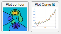
Use “scalable vector graphics” files for high-resolution images that are scaled to different sizes while preserving their shape and retaining their clarity. A quick and easy way to remember which plotting function is assigned to each button in an app is to assign an image of the plot to the button.

After creating the figure, expand the axes by setting the position or outerposition property to [0 0 1 1] in normalized units and save the figure using File > Save as and select svg format. Save the image to the folder containing your app. Then follow the same procedure as animated GIFs.

Display truecolor image

A truecolor image comes in the form of an [m x n x 3] array where each m x n pixel color is specified by an RGB triplet (read more) . This feature allows you to dynamically create a digital image or to upload an image from a mat file rather than an image file.

In this example, a progress bar is created within the uibutton callback function and it’s updated within a loop. For a complete demo of this feature see this comment .

% Button pushed function: ProcessDataButton
function ProcessDataButtonPushed(app, event)
    % Change button name to "Processing"
    app.ProcessDataButton.Text = 'Processing...';
    % Put text on top of icon
    app.ProcessDataButton.IconAlignment = 'bottom';
    % Create waitbar with same color as button
    wbar = permute(repmat(app.ProcessDataButton.BackgroundColor,15,1,200),[1,3,2]);
    % Black frame around waitbar
    wbar([1,end],:,:) = 0;
    wbar(:,[1,end],:) = 0;
    % Load the empty waitbar to the button
    app.ProcessDataButton.Icon = wbar;
    % Loop through something and update waitbar
    n = 10;
    for i = 1:n
        % Update image data (royalblue)
        % if mod(i,10)==0 % update every 10 cycles; improves efficiency
         currentProg = min(round((size(wbar,2)-2)*(i/n)),size(wbar,2)-2);
         RGB = app.ProcessDataButton.Icon;
         RGB(2:end-1, 2:currentProg+1, 1) = 0.25391; % (royalblue)
         RGB(2:end-1, 2:currentProg+1, 2) = 0.41016;
         RGB(2:end-1, 2:currentProg+1, 3) = 0.87891;
           app.ProcessDataButton.Icon = RGB;
          % Pause to slow down animation
          pause(.3)
          % end
      end
      % remove waitbar
      app.ProcessDataButton.Icon = '';
      % Change button name
      app.ProcessDataButton.Text = 'Process Data';
  end

The for-loop above was improved on Feb-11-2022.

Credit for the black & teal GIF icons: lordicon.com

David
David
Last activity on 23 May 2024

A colleague said that you can search the Help Center using the phrase 'Introduced in' followed by a release version. Such as, 'Introduced in R2022a'. Doing this yeilds search results specific for that release.
Seems pretty handy so I thought I'd share.

About Discussions

Discussions is a user-focused forum for the conversations that happen outside of any particular product or project.

Get to know your peers while sharing all the tricks you've learned, ideas you've had, or even your latest vacation photos. Discussions is where MATLAB users connect!

More Community Areas

MATLAB Answers

Ask & Answer questions about MATLAB & Simulink!

File Exchange

Download or contribute user-submitted code!

Cody

Solve problem groups, learn MATLAB & earn badges!

Blogs

Get the inside view on MATLAB and Simulink!

AI Chat Playground

Use AI to generate initial draft MATLAB code, and answer questions!