Deployment
Generate C/C++ code for prediction using a custom neural network architecture (requires MATLAB Coder and Deep Learning Toolbox)
You can generate C/C++ code for prediction using a custom neural network
architecture. In the call to fitcnet or
fitrnet,
specify the architecture using the Network name-value argument with
a dlnetwork (Deep Learning Toolbox) object. Save the resulting
model object using saveLearnerForCoder, and then load the model
in the prediction entry-point function using loadLearnerForCoder.
For an example that shows the code generation workflow, see Code Generation for Prediction of Machine Learning Model at Command Line.
Classification and Regression XGBoost Blocks: Simulate a model and generate code in Simulink
You can now integrate both the predict
function of the XGBoost regression objects and the predict
function of the XGBoost classification objects into Simulink® using the new XGBoost predict blocks. Import a trained model and configure
data types using the Block Parameters dialog box.
RegressionXGBoost Predict — This block predicts responses for new data using a trained XGBoost regression model (
CompactRegressionXGBoost).ClassificationXGBoost Predict — This block returns classified labels and predicted scores (optional) for new data using a trained XGBoost classification model (
CompactClassificationXGBoost).
Both blocks support C/C++ code generation and fixed-point conversion. You can generate C and C++ code using Simulink Coder™, and design and simulate fixed-point systems using Fixed-Point Designer™.
Classification and Regression Neural Network Blocks: Predict responses using a trained neural network model with a custom network architecture (requires Deep Learning Toolbox)
You can now import a trained neural network model with a custom network architecture from the MATLAB® workspace into a ClassificationNeuralNetwork Predict or RegressionNeuralNetwork Predict block to predict responses for new data.
At the MATLAB command line, train a neural network classification or regression model
with a complex architecture (such as a neural network with skip connections) using
fitcnet or
fitrnet.
Specify a layer array or a dlnetwork (Deep Learning Toolbox) object that contains the
network architecture by using the Network name-value argument of
the training function. Then import the trained model into Simulink, configure data types, and display the network architecture using the
Block Parameters dialog box.
Machine Learning Blocks: Predict responses using models trained on categorical predictors
The following Simulink machine learning prediction blocks now support models trained on matrix data that includes categorical predictors (tables are not supported):
Import a trained model from the MATLAB workspace into the block to predict responses for new data.
Apps
DOE Explorer App: Design systematic experiments and analyze response data
Use the DOE Explorer app to design a systematic experiment and analyze the effects of individual factors on a process response variable. Generate a full factorial, fractional factorial, response surface, or D-optimal design that is best suited for the types of factors and their expected interactions in your process of interest. After you generate a design, you can enter response data for the experimental design runs, or import the response data from a file or the MATLAB workspace. If you already have an experimental design, you can import it (and the response data) into the app for analysis.
Analyze your response data in the app by fitting a model to the response data using
regular or stepwise linear regression. The app computes error estimates and ANOVA
statistics for the model coefficients, and provides statistics and residual plots to
help you evaluate the goodness of fit. Create plots of main effects and interactions to
estimate the impact of individual factors and their interactions on the process
responses according to the model. You can also export the fitted regression model to the
workspace as a LinearModel object for further
analysis.
For more information about the app, see the DOE Explorer app reference page.
Gage R&R Analyzer App: Perform a gage repeatability and reproducibility study
Use the Gage R&R Analyzer app to perform a gage repeatability and reproducibility (R&R) study on a set of parts measurements made by different operators. After you import your measurement data from the workspace or a file into the app, you can set options such as the process specification limits, standard deviation multiplier, and ANOVA model type. The app performs an R&R study automatically and creates a bar chart and tables summarizing the gage and ANOVA model results. You can export the results to the MATLAB workspace for further analysis.
The app provides several charts to help you visualize your measurement data and the R&R study results:
Gage bar chart — Plot the relative contribution of different sources to the total measurement variance.
Control charts — Display Shewhart X-bar, R, and S control charts to show the measurements, specification limits, and out-of-control values.
Box chart — Display box charts of the measurement data and median values grouped by part, operator, or both.
Variability chart — Plot the individual measurements and their mean values for each operator and part.
For a workflow example, see Perform Interactive Gage Repeatability and Reproducibility Study.
For more details, see the Gage R&R Analyzer app reference page.
Machine Learning Apps: Import a trained XGBoost model
Import a supported trained XGBoost machine learning model into a Classification Learner or Regression Learner session in one of two ways:
On the Learn tab, in the File section, select Import Model > Import Trained Model from Workspace. See Import Trained Model into Current Session.
On the Learn tab, in the File section, select Import Model > Import Trained XGBoost Model from JSON File. See Import Trained XGBoost Model from JSON File.
After you import a trained model into the app, you can:
Assess model performance using a test data set.
Explain model behavior using interpretability plots.
Export the model for deployment.
For more information, see importModelFromXGBoost and Restrictions on Importing Models.
Machine Learning Apps: Create and train a model using custom neural network architecture (requires Deep Learning Toolbox)
You can now create and train a neural network model in Classification Learner or
Regression Learner using a custom network architecture with initialized or uninitialized
learnable parameters. In the Model Presets section of the
Learn tab, click Import Customizable Neural Network
from Workspace. Then select a dlnetwork (Deep Learning Toolbox) object from the workspace
to import its neural network into the model. After you create a draft customizable
neural network model, you can edit its network architecture, train the model and make
predictions using the app session data, and export the model to the workspace,
MATLAB
Coder, Simulink, or MATLAB
Production Server™. For more information, see Import Customizable Neural Network (Classification
Learner) and Import Customizable Neural Network (Regression
Learner).
Machine Learning Apps: Add model presets to create custom models
You can now add model presets to Classification Learner and Regression Learner to create custom machine learning models in the apps. In the Model Presets section of the Learn tab, click Add Custom Model Preset. Add MATLAB code to the template model class file to define the training function, prediction function, and hyperparameters of your machine learning model. Alternatively, you can use your own model class file. After you add a custom model preset to the app, you can use the model preset to create and train draft models in the current session and future app sessions. Click Manage Custom Model Presets in the Custom Models section of the Model Presets gallery to manage your custom model presets and export them from the app to share with other MATLAB users. For more information, see Add Custom Model Preset to Classification Learner and Add Custom Model Preset to Regression Learner.
Machine Learning Apps: View and export optimization results for optimizable models
When you train an optimizable model preset in Classification Learner or Regression Learner, you can now view a table of optimization results. On the Minimum Classification Error Plot tab (Classification Learner) or the Minimum MSE Plot tab (Regression Learner), select Table in the Show section to the right of the plot. The Optimization Iteration Results table displays the metrics and hyperparameter values for each optimization iteration. The table highlights the best point iteration and the iteration with the minimum observed error value. Export the optimization results to the MATLAB workspace by clicking Export Plot Data in the Export section of the Learn tab. For more information, see Hyperparameter Optimization in Classification Learner App and Hyperparameter Optimization in Regression Learner App.
.
Machine Learning Apps: Specify validation and test data set partitions
When you start a new Classification Learner or Regression Learner session by
importing data from the workspace or a data file, you can specify the validation scheme
and the indexing for the validation sets using a cvpartition object. In the Validation section of the
New Session dialog box, under Validation scheme, select
Use cvpartition object. Then select a
cvpartition object in the workspace. For more information, see
Select Validation Scheme in Classification Learner or Regression Learner.
In the same dialog box, you can also specify the rows in the data set to set aside as
test data using a cvpartition object. In the
Test section, select Set aside test data using a
cvpartition object and select a cvpartition object with
the type "holdout" in the workspace. For more information, see Test Trained Models in Classification Learner or Regression Learner.
Machine Learning Apps: Export trained customizable neural network model to Simulink or MATLAB Coder
After you train a customizable neural network machine learning model in Classification Learner or Regression Learner, you can now export the model directly to Simulink. You can then make predictions with the model in Simulink using new data, or using the exported predictor data from the app training data set. You can also export the model and sample predictor data from the app training data set to MATLAB Coder to generate C/C++ code. On the Learn tab, in the Export section, click Export and select Export Model to Simulink or Export Model to Coder.
Machine Learning Apps: Generate machine learning pipelines code
After you train a model in the Classification Learner or Regression Learner app, you can now generate machine learning pipelines code to create a pipeline that reproduces the data processing and model training steps. On the Learn tab, in the Export section, click Export and select Generate Pipeline Code from the Training Functions section. The generated code opens as a live script in the MATLAB editor.
Machine Learning
Incremental Learning: Train a neural network regression or classification model on incoming observations from streaming data, and assess performance in real time
You can create a neural network incremental learner for regression
(incrementalRegressionNeuralNetwork) or classification
(incrementalClassificationNeuralNetwork) in two ways:
Convert a traditionally trained model that is fit to a batch of data (
ClassificationNeuralNetworkorRegressionNeuralNetwork) to an incremental learner by passing the model to theincrementalLearnerfunction. Compact models and models that contain adlnetwork(Deep Learning Toolbox) object are not supported. The converted model is warm, meaning its property values reflect the knowledge gained from the traditionally trained model.If you do not have a supported, traditionally trained model, or you want to prepare an incremental learner to fit to data, call
incrementalRegressionNeuralNetworkorincrementalClassificationNeuralNetworkdirectly. A model created in this way is cold, but you can specify parameters from prior knowledge, such as network learnable values.
Regardless of how you create the model, you can perform these tasks in real time: train the model, assess the model's performance, and predict responses as the model accesses data, either per individual observation or per specified batch size.
The
fitfunction fits the model by updating the network learnables given an incoming batch of data.The
updateMetricsfunction evaluates the performance of the model as it processes incoming observations. The function writes specified metrics, measured cumulatively and within a designated window of processed observations, to theMetricsproperty of the model.The
updateMetricsAndFitfunction first evaluates the performance of the model by callingupdateMetricson incoming data, and then fits the model to that data by callingfit.The
predictfunction predicts responses given incoming predictor data.The
lossfunction returns the classification or regression loss given incoming predictor and response data. UnlikeupdateMetrics, thelossfunction does not write the computed loss to the model.The
perObservationLossfunction returns the per-observation loss.The
resetfunction resets all the learned parameters of the model. The function also resets the predictor mean and standard deviation property values, and the response mean and standard deviation property values (for a regression model), if these values are estimated by thefitfunction.
You can use the dlnetwork function to convert an
incrementalRegressionNeuralNetwork or
incrementalClassificationNeuralNetwork model object to a
dlnetwork object.
Compute the class-unweighted loss for classification models
You can compute the class-unweighted loss for classification models by setting the
Prior name-value argument to "empirical" in
the call to the loss object function. You can also compute a
class-weighted loss by setting Prior to the value
"uniform" or a numeric vector whose entries sum to
1.
The following functions support the new Prior name-value
argument:
| Classification Model | Function |
|---|---|
| Discriminant analysis classifier | loss |
| Multiclass model for support vector machines or other classifiers | loss |
| Ensemble of learners for classification | loss |
| Generalized additive model (GAM) | loss |
| Gaussian kernel classification model using random feature expansion | loss |
| k-nearest neighbor classifier | loss |
| Linear classification model | loss |
| Multiclass naive Bayes model | loss |
| Neural network classifier | loss |
| Support vector machine (SVM) classifier for one-class and binary classification | loss |
| Binary decision tree for multiclass classification | loss |
| XGBoost classification model | loss |
| All of the above | permutationImportance |
Create neural network template object
You can create a neural network template object by using the templateNeuralNetwork function. Pass the template object to testckfold to compare the accuracy of classification models, fitsemiself
to label data using semi-supervised learning, or directforecaster to fit a direct forecasting model.
Machine Learning Pipelines: Specify custom neural network architecture (requires Deep Learning Toolbox)
You can now use two new pipeline components to incorporate custom neural network
architectures into a machine learning pipeline. The
classificationCustomNeuralNetworkComponent and
regressionCustomNeuralNetworkComponent let you specify a dlnetwork (Deep Learning Toolbox) or layer array object as
the neural network architecture, giving you control over the network layers and
connections used for training and prediction within the pipeline.
Machine Learning Pipelines: Fit linear models, generalized linear models, and stepwise linear models in a pipeline
You can now create three new pipelines components for regression:
regressionLMComponent— Linear model for regressionregressionGLMComponent— Generalized linear model for regressionregressionStepwiseLMComponent— Linear model for stepwise regression
You can use these components to create and train regression models as
individual components or incorporated into a pipeline using the learn and
run object
functions.
Enhanced control over parallel execution with
UseParallel
You now have more control over when to use a parallel pool to execute supported
machine learning functions. The UseParallel name-value argument now
accepts new "off", "auto", or
"on" values. Specify UseParallel as
"auto" to automatically use a parallel pool if one is available or
as "on" to always use a parallel pool.
Starting in R2026b, specifying the UseParallel name-value
option as true or false is not recommended. For
more information see Logical values for UseParallel argument not recommended.
Functionality being removed or changed
Logical values for UseParallel argument not
recommended
Behavior change
Starting in R2026b, specifying the UseParallel name-value
argument as true or false is not recommended.
Use "off", "auto", or "on"
values instead.
This table shows how to update your code depending on your goal.
| Goal | Not Recommended | Recommended |
|---|---|---|
Write code that runs on the MATLAB client. |
UseParallel=false
|
UseParallel="off"
|
| Write portable code that runs on a parallel pool and, if a pool is not available, runs on the MATLAB client. |
UseParallel=true
|
UseParallel="auto"
|
| Write code that runs on a parallel pool and errors if a pool is not available. | N/A |
UseParallel="on"
|
There are no plans to remove support for the true
or false values.
Statistics
Design of Experiments: Create a responseSurfaceDOE object to
generate an experiment design
Generate a response surface experiment design by using the responseSurfaceDOE function to create an object of the same name. You can
create a central composite (Box–Wilson) or Box–Behnken design that is suitable for
calibrating a quadratic model of a curved response surface. The object properties
include information about the design, model, and factors used to generate the design.
After creating the object, you can use the fitlm
function to fit a linear model to the design points.
Design of Experiments: Add replicates to a design of experiments object
Add one or more replicates to a design of experiments object using the addReplicates
function. A replicate is a duplicate of the original design runs in the object when it
is created. For a list of design of experiments objects, see Design of Experiments (DOE).
Design of Experiments: Randomize the run order of a design of experiments object
Randomize the run order of a design of experiments object using the randomizeRunOrder function. For a list of design of experiments objects,
see Design of Experiments (DOE).
capability and capaplot Functions: Specify a
continuous probability distribution
You can now compute capability indices and create capability plots using a
probability distribution other than the normal distribution. Specify the name of a
continuous probability distribution supported by the fitdist function in the call to the capability or capaplot function. Alternatively, you
can specify the name of a continuous probability distribution object in the workspace.
When you specify a nonuniform probability distribution in the call to the
capability function, you can use the IndexEstimationMethod name-value argument to choose the capability index
estimation method, either percentile or z-score.
capability Function: Compute confidence intervals for capability
indices
The capability function now returns
confidence intervals for the capability indices in the output structure S. To
specify the significance level for the confidence intervals, use the Alpha
name-value argument. If you specify a nonuniform probability distribution, the function
computes the confidence intervals using a bootstrap method. You can set the number of
bootstrap iterations using the NumBootstrapSamples name-value argument.
Probability Distributions: Create shifted exponential, gamma, and Weibull distribution objects
You can create three new shifted probability distribution objects using makedist, or by fitting data with fitdist or the Distribution Fitter app:
ShiftedExponentialDistribution— Two-parameter Exponential DistributionShiftedGammaDistribution— Three-parameter Gamma DistributionShiftedWeibullDistribution— Three-parameter Weibull Distribution
Each object includes a location parameter theta such that the
distribution starts at x=theta instead of zero. You can use the
objects with generic functions such as pdf, cdf, and random.
pdist2 Function: Use tables for input data and compute distances
for categorical and mixed data
You can now use tables to provide input data to the pdist2 function when computing pairwise distances. Specify which
variables to include in the computation by using the VariableNames
name-value argument.
You can now compute the pairwise distance between data sets containing categorical or
mixed data. Specify categorical variables using the
CategoricalVariables name-value argument.
Enhanced control over parallel execution with
UseParallel
You now have more control over when to use a parallel pool to execute supported
statistics functions. The UseParallel name-value argument now
accepts new "off", "auto", or
"on" values. Specify UseParallel as
"auto" to automatically use a parallel pool if one is available or
as "on" to always use a parallel pool.
Starting in R2026b, specifying the UseParallel name-value
option as true or false is not recommended. For
more information see Logical values for UseParallel argument not recommended.
Functionality being removed or changed
Logical values for UseParallel argument not
recommended
Behavior change
Starting in R2026b, specifying the UseParallel name-value
argument as true or false is not recommended.
Use "off", "auto", or "on"
values instead.
This table shows how to update your code depending on your goal.
| Goal | Not Recommended | Recommended |
|---|---|---|
Write code that runs on the MATLAB client. |
UseParallel=false
|
UseParallel="off"
|
| Write portable code that runs on a parallel pool and, if a pool is not available, runs on the MATLAB client. |
UseParallel=true
|
UseParallel="auto"
|
| Write code that runs on a parallel pool and errors if a pool is not available. | N/A |
UseParallel="on"
|
There are no plans to remove support for the true
or false values.
Visualization
capaplot Function: Display a data histogram in the capability
plot
Display a data histogram in the capability plot by specifying
ShowHistogram=true in the call to capaplot.
confusionchart Function: Display or hide axes toolbar of a
confusion chart
Display or hide the axes toolbar of a ConfusionMatrixChart object by
setting the ToolbarVisible property. The axes toolbar is visible by
default, but you can hide it by setting the property to "off".
To create a confusion chart, use the confusionchart function. For more information about how to set these
properties, see ConfusionMatrixChart Properties.
variabilitychart Function: Visualize data variability across
factors using variability charts
Use the variabilitychart function to create variability charts
that show how data varies across different factors. Variability charts help you identify
where variation originates and understand what drives differences in a process. You can
customize the chart with boxes, mean lines, colored factor levels, and target value
lines.
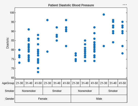
variabilitychart Function: Visualize data variability across factors using variability charts